Steady and Unsteady state analysis of 2D Heat conduction equation
2D Heat conduction Steady and Transient state analysis.
The equation in general is given as : `(delT)/(delt) + alpha*((del^2T)/(delx^2) + (del^2T)/(dely^2)) = 0`
Steady state : The steady state 2D heat conduction is given as : `(del^2T)/(delx^2) + (del^2T)/(dely^2) = 0`
Unsteady/Transient state : `(delT)/(delt) + alpha*((del^2T)/(delx^2) + (del^2T)/(dely^2)) = 0`
We need to discretize these equations to solve them. Hence for steady state equation:
`(del^2T)/(delx^2) + (del^2T)/(dely^2) = 0`
`(T_L+2*T_P+T_R)/(delx^2) + (T_T-2*T_P+T_B)/(dely^2) = 0` ....second order approximation.
where `T_T = T(i,j+1) , T_B = T(i,j-1) , T_L = T(i-1,j) , T_R = T(i+1,j)`
`therefore` `2*(T_P)/(delx^2) + 2*(T_P)/(dely^2) = (T_L+T_R)/(delx^2) + (T_T+T_B)/(dely^2)`
`therefore` `T_P*(2*(delx^2+dely^2))/((delx^2)*(dely^2)) = (T_L+T_R)/(delx^2) + (T_T+T_B)/(dely^2)`
take k = `(2*(delx^2+dely^2))/((delx^2)*(dely^2))`
`therefore T_P = 1/k*((T_L+T_R)/(delx^2)) +1/k*((T_T+T_B)/(dely^2))`
========================================================================
Unsteady state :
the equation in discretized form is given as : `(T_(i,j)^(n+1)-T_(i,j)^(n))/(delt) + alpha*((del^2T)/(delx^2) + (del^2T)/(dely^2)) = 0`
Since the second half of the above equation is elliptic in nature, we consider points from both the neighbouring points.
`therefore (T_(i,j)^(n+1)-T_(i,j)^(n))/(delt) + alpha* [(T_(i+1,j)-2*T_(i,j)+T_(i-1,j))/(delx^2) + (T_(i,j+1)-2*T_(i,j)+T_(i,j-1))/(dely^2)]`
.........at nth time step.
considering `T_T = T(i,j+1) , T_B = T(i,j-1) , T_L = T(i-1,j) , T_R = T(i+1,j)`
`therefore T_(i,j)^(n+1) = T_(i,j)^n + alpha*delt*[(T_R-2*T_P+T_L)/(delx^2) + (T_T-2*T_P+T_B)/(dely^2)]` ..... at nth time step.
this is called as explicit form of the equation.
the same equation is given in implicit form as : `T_(i,j)^(n+1) = T_(i,j)^n + alpha*delt*[(T_R-2*T_P+T_L)/(delx^2) + (T_T-2*T_P+T_B)/(dely^2)]` .............. at (n+1)th time step.
to further simplify it let us manipulate it,
Let `k1 = alpha*(delt)/(delx^2) and k2 = alpha*(delt)/(dely^2)`
`T_P^(n+1) = T_P^n + k1*(T_L^(n+1)-2*T_p^(n+1)+T_R^(n+1)) + k2*(T_T^(n+1)-2*T_P^(n+1)+T_B^(n+1))`
`therefore T_P^(n+1)*(1+2k1+2k2) - k1*T_L^(n+1) - k1*T_R^(n+1) - k2*T_T^(n+1)-k2*T_B^(n+1) = T_P^n`
`T_P^(n+1) = [T_P^n + k1*T_L^(n+1)+k1*T_R^(n+1)+k2*T_T(n+1)+k2*T_B^(n+1)]/(1+2k1+2k2)`
we solve this equation iteratively, the value for `T_P^(n)` doesnt change within the iteration and the other values of T at right side of equation change within iteration. This is for implicit case.
==========================================================================
Steady state : The code is as follows :
clc
close all
clear all


L = 1;
nx = 10;
ny = 10;
dx = L/(nx-1);
dy = L/(ny-1);
dt = 1e-2;
x = linspace(0,1,nx);
y = linspace(0,1,ny);
[xx,yy] = meshgrid(x,y)
%zz = [xx,yy]
% initial and boundary conditions
T = 300*ones(nx);
T(1:ny,1) = 400;  %left
T(1,1:nx) = 600;  %top
T(ny,1:ny) = 900; %right
T(1:nx,nx) = 800; %bottom
T(1,1) = 500;
T(1,nx) = 750;
T(ny,1) = 650;
T(nx,ny) = 850;

Told = T
k = 2*(((dx)^2+(dy)^2)/((dx^2)*(dy^2)));
% steady state 2D heat conduction
% Explicit
% Jacobi
error = 1;
tol = 1e-4
iterative_solver = 1

% code for jacobi iterative solver

if iterative_solver == 1
 tic
   jacobi_iter = 1
    while error > tol;
    for i = 2:nx-1
        for j = 2:ny-1
            %[T(i,j)] = steady_explicit(dx(i),dy(j),k,Told)
            term1 = 1/k*((Told(i-1,j) + Told(i+1,j))/(dx^2));
            term2 = 1/k*((Told(i,j+1)+Told(i,j-1))/(dy^2));
            T(i,j) = term1 + term2;
        end
    end
    error = max(max(abs(Told - T)));
    Told = T;
    jacobi_iter = jacobi_iter + 1
    jtime = toc

    end


    figure(1)
    contourf(xx,yy,T);
    colormap(jet)
    colorbar
    xlabel('X-axis')
    ylabel('Y-axis')
    ax = gca;
    ax.YDir = 'reverse';
    title_text = sprintf('Jacobi iteration no = %d',jacobi_iter);
    title_text2 = sprintf('Iteration time = %d',jtime);
    title(title_text,title_text2);
end


%% code for gauss seidel solver
if iterative_solver == 2
    tic
    gs_iter = 1
    while error > tol;
    for i = 2:nx-1
        for j = 2:ny-1
            %[T(i,j)] = steady_explicit(dx(i),dy(j),k,Told)
            term1 = 1/k*((T(i-1,j) + Told(i+1,j))/(dx^2));
            term2 = 1/k*((T(i,j+1)+Told(i,j-1))/(dy^2));
            T(i,j) = term1 + term2;
        end
    end
    error = max(max(abs(Told - T)))
    Told = T;
    gs_iter = gs_iter + 1
    gstime = toc


    end

    figure(2)
    contourf(xx,yy,T);
    colormap(jet)
    colorbar
    xlabel('X-axis')
    ylabel('Y-axis')
    ax = gca;
    ax.YDir = 'reverse';

    title_text = sprintf('Gauss Seidel iteration no = %d',gs_iter);
    title_text2 = sprintf('gs_iteration time = %d',gstime);
    title(title_text,title_text2);
end


%% SOR approach

if iterative_solver == 3
tic

 w = 1.1
 sor_iter = 1
    while error > tol;
    for i = 2:nx-1
        for j = 2:ny-1
            term1 = 1/k*((T(i-1,j) + Told(i+1,j))/(dx^2));
            term2 = 1/k*((T(i,j+1)+Told(i,j-1))/(dy^2));
            T(i,j) = term1 + term2;
            T(i,j) = ((1-w)*Told(i,j)) + (w*T(i,j));
        end
    end
    error = max(max(abs(Told - T)))
    Told = T;
    sor_iter = sor_iter + 1
    sortime = toc

    end

    figure(3)
    contourf(xx,yy,T);
    colormap(jet)
    colorbar
    xlabel('X-axis')
    ylabel('Y-axis')

    title_text = sprintf('sor iteration no = %d',sor_iter);
    title_text2 = sprintf('iteration time = %d',sortime);
    title(title_text,title_text2);
    ax = gca;
    ax.YDir = 'reverse';
end


% time = [jtime,gstime,sortime]
% figure(3)
% bar(time,0.40,'green')
% xticklabels({'jtime','gstime','sortime'});
% title('time comparison');


% bar graph for iteration comparison
% iteration = [jacobi_iter,gs_iter,sor_iter]
% figure(3)
% bar(iteration,0.40,'green')
% xticklabels({'jacobi_iter','gs_iter','sor_iter'})
% title('iteration comparison')
%
the result and iteration comparison graph is given as follows :
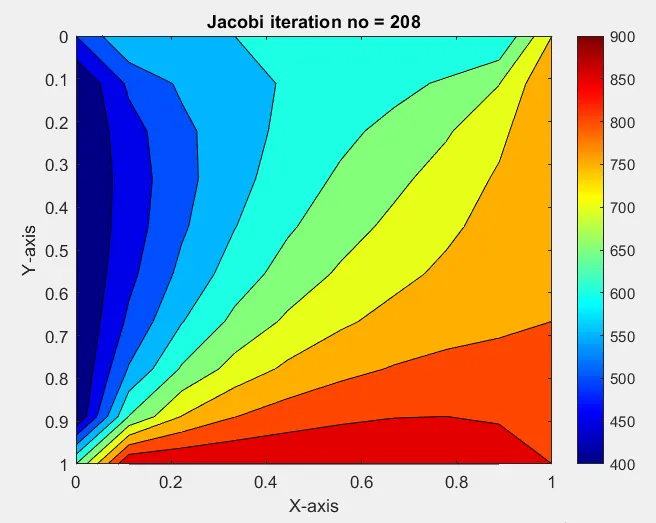
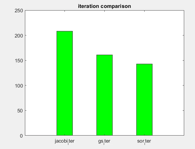
As we can see from the bar graph the iterations taken by the SOR method is lowest than the other methods. As the SOR method uses an aggressive step to calculate the next T values in order to converge. It is not always beneficial to use the SOR method as in some cases it might overshoot the assumption and it might take longer no. of iterations to come back to the required converged result.
the value of 'w' determines whether the solution would be over-relaxed (w>1) or under-relaxed (w<1).
Unsteady implicit state equation :
the code is as follows :
% Unsteady state solver, implicit method.
clc
close all
clear all


L = 1;
t = 300;
nx = 20;
ny = 20;
alpha = 1.4;
dx = L/(nx-1);
dy = L/(ny-1);
dt = 1e-3;
%nt = t/dt;
nt = 1000
x = linspace(0,1,nx);
y = linspace(0,1,ny);
[xx,yy] = meshgrid(x,y);
k1 = alpha*dt/(dx^2);
k2 = alpha*dt/(dy^2);


% initial and boundary conditions
T = 300*ones(nx);
T(1:ny,1) = 400;  %left
T(1,1:nx) = 600;  %top
T(ny,1:ny) = 900; %right
T(1:nx,nx) = 800; %bottom
% temperature at corners taken as the average of the adjacent walls
T(1,1) = 500;
T(1,nx) = 750;
T(ny,1) = 650;
T(nx,ny) = 850;
term1 = 1/(1+(2*k1)+(2*k2));
term2 = k1*term1;
term3 = k2*term1;
error = 9e9;
tol = 1e-4;
% initialize
Told = T;
Tprev = T;

% unsteady explicit
iterative_solver = 3    % the no. to this command can be changed to avail the required solver.

% Jacobi solver
if iterative_solver == 1
    jacobi_iter = 1;
   tic
 % time loop
 for m = 1:nt;
     error = 9e9;
     while error > tol
        %space loop
        for i = 2:nx-1
            for j = 2:ny-1
                T(i,j) = term1*Tprev(i,j) + term2*(Told(i-1,j)+Told(i+1,j)) + term3*(Told(i,j+1)+Told(i,j-1));
            end
        end
        error = max(max(abs(Told-T)));
        Told = T;
        jacobi_iter = jacobi_iter +1;
     end
     Tprev = T
end
jacobi_time = toc


    figure(1)
    contourf(xx,yy,T);
    colormap(jet);
    colorbar;
    xlabel('X-axis');
    ylabel('Y-axis');
    ax = gca;
    ax.YDir = 'reverse';
    title_text = sprintf('jacobi iteration no = %d',jacobi_iter);
    title_text1 = sprintf('jacobi time = %d',jacobi_time);
    title(title_text);
    title(title_text1,title_text);
end


%% G-S solver
if iterative_solver == 2
    gs_iter = 1;
   tic
 % time loop
 for m = 1:nt;
     error = 9e9;
     while error > tol
        %space loop
        for i = 2:nx-1
            for j = 2:ny-1
                T(i,j) = term1*Tprev(i,j) + term2*(T(i-1,j)+Told(i+1,j)) + term3*(T(i,j+1)+Told(i,j-1));
            end
        end
        error = max(max(abs(Told-T)));
        Told = T;
        gs_iter = gs_iter +1;
     end
     Tprev = T;
end
gs_time = toc

    figure(1)
    contourf(xx,yy,T);
    colormap(jet);
    colorbar;
    xlabel('X-axis');
    ylabel('Y-axis');
    ax = gca;
    ax.YDir = 'reverse';
    title_text = sprintf('GS iteration no = %d',gs_iter);
    title_text1 = sprintf('GS time = %d',gs_time);
    title(title_text,title_text1);
end


%% SOR method solver

if iterative_solver == 3

 w = 1.2
 sor_iter = 1
 tic
 for m = 1:nt;
     error = 9e9;
     tol = 1e-4;
    while error > tol;

    for i = 2:nx-1
        for j = 2:ny-1
            T(i,j) = term1*Tprev(i,j) + term2*(T(i-1,j)+Told(i+1,j)) + term3*(T(i,j+1)+Told(i,j-1));
            T(i,j) = ((1-w)*Told(i,j)) + (w*T(i,j));
        end
    end
    error = max(max(abs(Told - T)))
    Told = T;
    M(sor_iter)=getframe(gcf);
    sor_iter = sor_iter + 1;


    end
    Tprev = T;


 end
sor_time = toc;

    figure(1)
    contourf(xx,yy,T);
    colormap(jet)
    colorbar
    xlabel('X-axis')
    ylabel('Y-axis')


    title_text = sprintf('sor iteration no = %d',sor_iter);
    title_text1 = sprintf('SOR time = %d',sor_time);
    title(title_text,title_text1);
    ax = gca;
    ax.YDir = 'reverse';
    grid on
end


%      movie(M)
%      videofile = VideoWriter('Unsteady Implicit SOR.avi','Uncompressed AVI');
%      open(videofile)
%      writeVideo(videofile,M)
%      close(videofile)


%bar graph for iteration comparison
% iteration = [jacobi_iter,gs_iter,sor_iter]
% figure(3)
% bar(iteration,0.40,'green')
% xticklabels({'jacobi_iter','gs_iter','sor_iter'})
% title('iteration comparison')
the result and the bar graph comparison for all 3 iteration methods is given as follows :
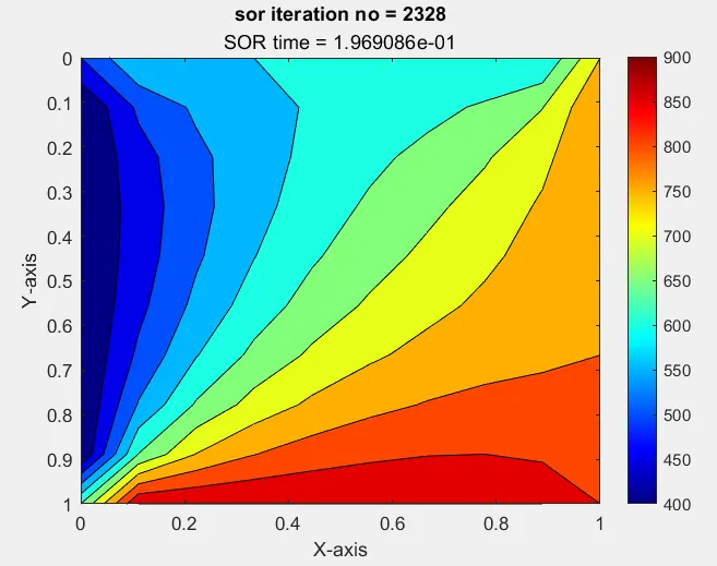
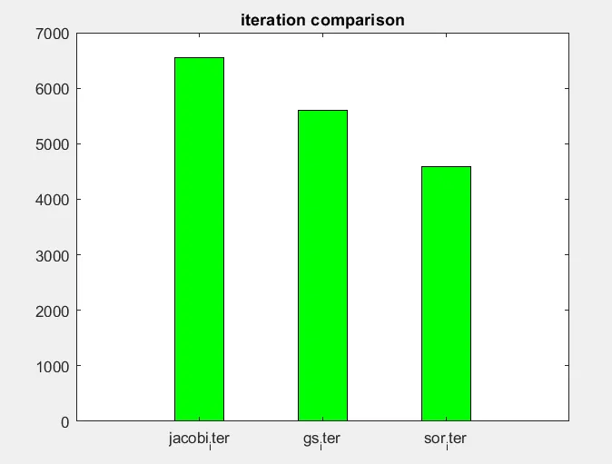
As we can see from the above graph, again the iteration taken to converge the solution for SOR method is lowest in comparison to the other methods.
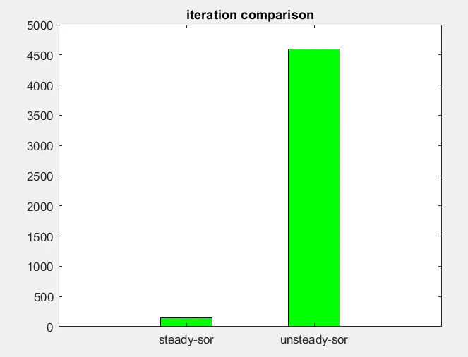
Comparing the SOR method comparison between the steady and unsteady implicit state :
============================== end ==================================