stalagmite function

AIM: To write a code to optimize the stalagmite function and find the global maxima of the function.

Description:

Genetic algorithms are search algorithms based on the mechanics of natural selection and natural genetics. The main goal to develop search algorithms is to abstract and rigorously explain the adaptive process of natural systems and to design artificial systems software that retains the important mechanisms of natural systems. If such artificial systems are made more robust,costly redesign can be reduced or eliminated. The more the adaptation ,the more better performance can be expected.Since the genetic algorithms are computationally simple yet powerful ,efficient and effective searching procedure in many complex environments, has become widespread application in business, scientific and engineering circles.

How it works?

GA’s work with a coding of the parameter set, not the parameters themselves.

GA’s search from a population of points, not a single point

GA’s use objective function information, not derivatives or other auxillary knowledge

GA’s use probabilistic transition rules

Optimisation:

Optimisation is necessary when we are looking for perfection .It studies how to describe and attain the best. Thus the optimization seeks to improve performance toward some optimal point or points.

The mechanics of a simple genetic algorithm are surprisingly simple, involving nothing more complex than taking elments from populationand execute through a fitness function. A genetic algorithm starts with a population of elements and thereafter generates successive population of elements. By working from a population of well adapted diversity instead of single point, the genetic algorithm adheres to the old proverb that there is safety in numbers. GAs takes blindly the objective function values associated with individual element. Direct use of a coding, search from a population, blindness to auxiliary information, and randomized operators contribute to a genetic algorithm’s robustness and resulting advantage over other more commonly used techniques.

The three operators uses by GAs are

1. Reproduction
2. Crossover
3. Mutation

Reproduction is a process in which individual points/elements are taken according to their objective function values, f the biologists call this function the fitness function. Taking values of elements according to their fitness values means that elements with a higher value have a higher probability of contributing one or more of its properties in the next generation, a Darwinian survival of the fitness among element creatures. In natural population fitness is determined by a creature’s ability to survive to adulthood and subsequent reproduction. In this artificial setting objective function is the final decision maker of the individual creature’s life and death. Once an individual has been selected for reproduction, an exact replica of the individual is made. This individual is then entered into a mating pool, a tentative new population, for further genetic operator action.

After reproduction, simple crossover may proceed in two steps. First members of the newly reproduced elements in the mating pool are mated at random. Second each pair of elements undergoes crossing over . The process of reproduction and crossover in a genetic algorithm is a kind of exchange. High performance elements are repeatedly tested and exchanged in the search for better and better performance .

Mutation palys a secondary role in the operations of genetic algorithm. Mutation is needed because even though reproduction and crossover effectively search and recombine extant properties, sometimes we lose some potential useful genetic material. The mutation operator protects against such an irrecoverable loss.

Life cycle of Genetic Algorithm :

Objective:

Consider the function for a problem,

`f(x,y)= f1x *f2x *f1y*f2y`

`f1x=[sin(5.1pix+0.5)]^6`

`f1y=[sin(5.1piy+0.5)]^6`

`f2x=exp[-4ln(2)(x-0.0667)^2/0.64]`

`f2y=exp[-4ln(2)(y-0.0667)^2/0.64]`

Initially to use genetic algorithm, we have to code the decision variables of our problem as some finite- length . Here

x=linspace(0,0.6,150)

y=linspace(0,0.6,150)

We select an initial population at random and presented along with the fitness or objective function values f(x,y).

The fitness function will accept a vector x of size 1-by-nvars (nvars=2) and returns a scalar evaluated at x i.e. ,input_vector is a row vector . The fitness function competes the values of the function and returns that scalar value as argument [f] which will be minimum or maximum values.

function [f]=get_stalagmite(input_vector)


x1=input_vector(1);
y1=input_vector(2);
f1x=(sin(5.1*pi*x1+0.5))^6
f1y=(sin(5.1*pi*y1)+0.5)^6
f2x=exp((-4)*log(2)*((x1-0.0667)^2/0.64))
f2y=exp((-4)*log(2)*(y1-0.0667)^2/0.64)

[f]=-(f1x*f1y*f2x*f2y);
end

Here we modified the function ,f=-f becuase the output values plotted are the minimum values. In order to get maximum values we modify the stalagmite function with -sign.

The solver we use here is ' ga ' genetic algorithm which have nothing to do with the information given above but optimize the fitness function . It generates population of points at each iteration. The best point in the population approaches an optimal solution.

Here we did three observations

Study1: Study of statistical behaviour of elements with no bounds. It means the population of parameter set can be taken beyond the defined bounds. It may take beyond o.6 or under 0 values. The number of cases taken by the solver to run fitness function is 50.

• x and y are row vectors of size 1X 150.we have taken 150 values between the limits 0 to 0.6 and are passed as input parameters
• using Meshgrid command , the values from x and y row vectors are taken and generates grid of 2d vectors(150X150) values
• from this 2d vectors xx and yy , each row is taken as input parameter and passed into the fitness function.i.e., input_vector(1), input_vector(2).
• using for loop the fitness function generates 150 population of scalar values or parameters ,f as output.
• These f values and their corresponing x and y values are taken by solver ga and executes the optimal value.

clear all
close all
clc

%defining our search space
x=linspace(0,0.6,150);
y=linspace(0,0.6,150);


[xx,yy]=meshgrid(x,y);

for i=1:length(xx)
    for j=1:length(yy)

input_vector(1)=xx(i,j);
input_vector(2)=yy(i,j);
f(i,j)=get_stalagmite(input_vector);

    end
end


%study1_stalagmite behaviour
tic
num_cases=50
for i=1:num_cases
    
    [ inputs,fopt(i)]=ga(@get_stalagmite,2);
    xopt(i)=inputs(1);
    yopt(i)=inputs(2);
       
end
study1_time=toc

figure(1)
subplot(2,1,1)
hold on
surfc(x,y,-f)
shading interp
plot3(xopt,yopt,-fopt,'marker','o','markersize',5,'markerfacecolor','r')
title('unbounded inputs')
subplot(2,1,2)
plot(-fopt)
xlabel('Iterations')
ylabel('Function Minimum')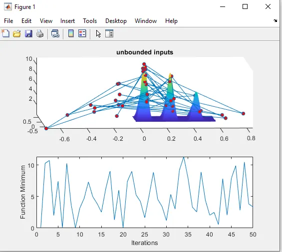

Using tic and toc command we can see the time taken to run the code. study time for this code is 100 sec. we can minimise this study time by giving bounds to data set.

Study2: Study of statistical behaviour of elements with upper and lower bounds.

• To minimise the fitness function using ga,pass a function handle to the fitness function as well as the number of variables in the problem
• The lower and upper bounds given are [0;0],[1;1] and pass the bounds as the fifth and sixth argumens after the number of variables.
• fval is the value of the function get_stalagmite evaluated at the point x.
• by using this method of passing function handlers,the time taken by the solver also reduces
• study2_time is 70 sec which is lesser than the previous one.
• [],[].. are actually inbuilt functions of genetic algorithm solver ga. plotfunction ,output function...mostly takes empty values or zero value.

  %study2-statistical behaviour with upper and lower bounds
  tic
  for i=1:num_cases
      
      [inputs,fopt(i)]=ga(@get_stalagmite,2,[],[],[],[],[0;0],[1;1]);
      xopt(i)=inputs(1);
      yopt(i)=inputs(2);
  
  end
  study2_time=toc
  
  figure(2)
  F =-f
  subplot(2,1,1)
  hold on
  surfc(x, y, F)
  shading interp
  plot3(xopt,yopt,-fopt,'marker','o','markersize',5,'markerfacecolor','r')
  title('bounded inputs')
  subplot(2,1,2)
  plot(-fopt)
  xlabel('Iterations')
  ylabel('Function Maximum')​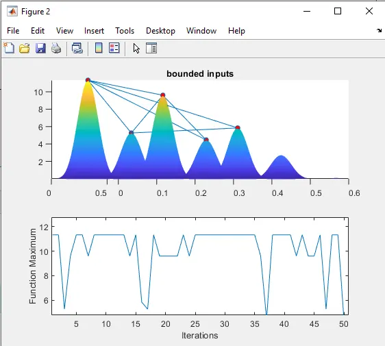

  

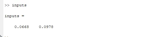
Output: Maximum peak position ,x and y.

study3: study by increasing GA iterations.

• By increasing iterations we can optimise the solution.
• here the iterations has increased to 170.

• %study 3 increasing GA iterations
  options=optimoptions('ga')
  options=optimoptions(options,'populationsize',170);
   tic
   for i=1:num_cases
       [ inputs, fopt(i)]=ga(@stalagmite,2,[],[],[],[],[0;0],[1;1],[],[],options);
       xopt(i)=inputs(1);
       yopt(i)=inputs(2);
   end
   study3_time=toc
   figure(3)
   subplot(2,1,1)
   hold on
  surfc(x, y, -f)
  shading interp
  
  plot3(xopt,yopt,-fopt,'marker','o','markersize',5,'markerfacecolor','r')
  title('bounded inputs')
  subplot(2,1,2)
  plot(-fopt)
  xlabel('Iterations')
  ylabel('Function Minimum')​

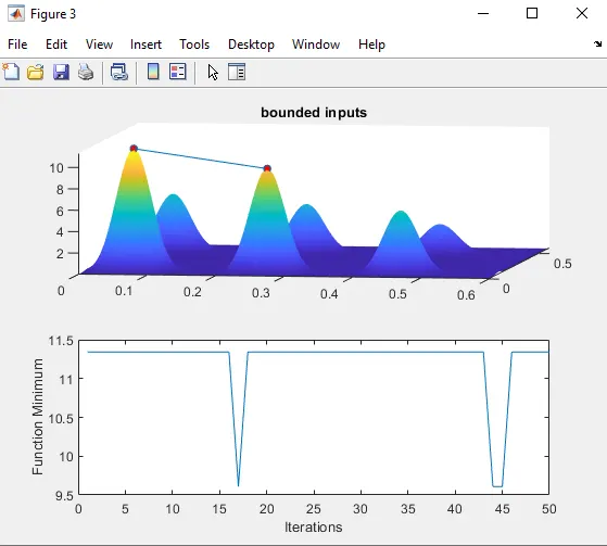
The above plot shows that the minimal values are obtained at 11.4 and study time it took 3 times more than first study.

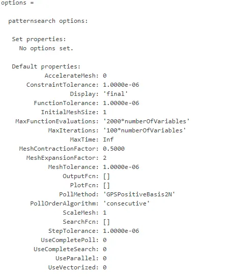
Optimsation options affect how a solver behaves and can monitor the progress of function by setting options. Here optimevalue taken as 'populationsize'. The following details below shows the properties we can set as options for a solver to get better result.

Conclusion: Using Genetic algorithm we can solve many complex problems in different fields of science.