Curve Fitting

AIM: To write a code to fit a linear or cubic polynomial for a Cp data .

Description :

How to make the curve perfectly?

A: Curve Fitting: The process of constructing a curve or mathematical function that has the best fit to a series of data points ,possibly subject to constraints. It can involve interpolation where an extrafit to the data is required or smoothing in which a smooth function is constructed that approximately fit the data.

polyval: it is matlab function that computes a least square polynomials for a given set of data.

polyfit: It generates the coefficients of the polynomial,which can be used to model a curve to fit the data.

How to determine which fit is best?

A: we have two methods to determine the best fit

1. Graphical fit
2. Numerical fit

Graphical Fit: we can determine the best fit by comparing the graphs of different fits simultaneously. sometimes the fits and residuals (the difference betten original date and predicted dta points are shown) for the polynmials are all similar making it difficult to choose the best one.

Numerical Fit: when u cannot longer eliminate fits by examining them graphically,we can evaluate by examining numerical fit results. The curve fitting tool displays two types of numerical fit results

• Goodness-of-fit statistics
• Confidence bounds on the fitted coefficients

The goodness-of-fit statistics help to determine how well the curve fits the data. The confidence bounds on the coefficients determine their accuracy.

Goodness-of-fit statistics help to determine how well the model fits the data. The parameters we use to determine the fitness characteristics for any degree curve are-

1. SSE is the sum of squares due to error of the fit. A value closer to zero indicates a fit that is more useful for prediction
2. R-Square is the square of the correlation between the response values and the predicted response values. A value closer to 1 indictes that a greater proportion of variance is accounted for by the model.
3. DFE is the degree of freedom in the error
4. Adj R-sq is the degrees of freedom adjusted R-square. A value closer to 1 indicates a better fit
5. RMSE is the root mean square error. A value closer to 0 indicates a fit that is more useful for prediction
6. #coeff is the number of coefficients in the model. When we have several fits with similar goodness-of-fit statistics, look for the smallest number of coefficients which help to decide which fit is best

we need to take different orders of polynomial equations for the same data for to determine the best fit and observe all the above mentioned Goodness-of-fit parameters

Examine the values of sum of squares due to error(SSE) and the adjusted R-square statistics helps to determine the best fit. The SSE statistic is the least squares error of the fit, with a value closer to zero determines a better fit. The adjusted R-square statistic is generally the best indicator fit when we add additional coefficients to the model.

The coefficient bounds on the coefficients determine their accuracy

How to improve Cubic curve ?

A: we can improve the cubic curve fit by doing scaling and centering method which is called Normalisation using curve fitting tool in matlab.It removes the warning message and give the result with different coefficients .But the functional form of the data and the resulting goodness-of-fit statistics do not change. The data displayed in the curve fitting tool plots uses original scale.

Normalisation means analysing data without using units and measurments. we cannot use this data for comparing with non normalised data.

The other method we can use is splitwise method.The data is splited into equal fragments of data and polynomial equations of same or different order can be applied for each fragmentof data and can improve the curve fitting.

code for different fits for the same data:

clear all
close all
clc
 %preparing the data
 Cp_data=load('data');
 temperature=Cp_data(:,1);
 Cp=Cp_data(:,2);
 
 
%curve fit
%Cp=a*T^3+b*T^2+C*T+D
co_effs1=polyfit(temperature,Cp,1)
predicted_Cp1=polyval(co_effs1,temperature);

co_effs2=polyfit(temperature,Cp,2)
predicted_Cp2=polyval(co_effs2,temperature);

co_effs3=polyfit(temperature,Cp,3)
predicted_Cp3=polyval(co_effs3,temperature);

co_effs4=polyfit(temperature,Cp,4)
predicted_Cp4=polyval(co_effs4,temperature);

co_effs5=polyfit(temperature,Cp,5)
predicted_Cp5=polyval(co_effs5,temperature);

co_effs6=polyfit(temperature,Cp,6)
predicted_Cp6=polyval(co_effs6,temperature);

co_effs7=polyfit(temperature,Cp,7)
predicted_Cp7=polyval(co_effs7,temperature);

co_effs8=polyfit(temperature,Cp,8)
predicted_Cp8=polyval(co_effs8,temperature);

co_effs10=polyfit(temperature,Cp,10)
predicted_Cp10=polyval(co_effs10,temperature);

%compare any curve fit with the original data
figure(1)
plot(temperature,Cp,'linewidth',3)
hold on
plot(temperature,predicted_Cp1,'linewidth',3,'color','r')
xlabel('Temperature[K]')
ylabel('Specific Heat[kj/mol-k]')
legend('Original Dataset','linear Curve Fit')

figure(2)
plot(temperature,Cp,'linewidth',3)
hold on
plot(temperature,predicted_Cp2,'linewidth',3,'color','g')
xlabel('Temperature[K]')
ylabel('Specific Heat[kj/mol-k]')
legend('Original Dataset','quadratic Curve Fit')

figure(3)
plot(temperature,Cp,'linewidth',3)
hold on
plot(temperature,predicted_Cp3,'linewidth',3,'color','y')
xlabel('Temperature[K]')
ylabel('Specific Heat[kj/mol-k]')
legend('Original Dataset','cubic Curve Fit')

figure(4)
plot(temperature,Cp,'linewidth',3)
hold on
plot(temperature,predicted_Cp4,'linewidth',3,'color','#A2142F')
xlabel('Temperature[K]')
ylabel('Specific Heat[kj/mol-k]')
legend('Original Dataset','4th order Curve Fit')

figure(5)
plot(temperature,Cp,'linewidth',3)
hold on
plot(temperature,predicted_Cp5,'linewidth',3,'color','c')
xlabel('Temperature[K]')
ylabel('Specific Heat[kj/mol-k]')
legend('Original Dataset','5th orderCurve Fit')

figure(6)
plot(temperature,Cp,'linewidth',3)
hold on
plot(temperature,predicted_Cp6,'linewidth',3,'color','m')
xlabel('Temperature[K]')
ylabel('Specific Heat[kj/mol-k]')
legend('Original Dataset','6th order Curve Fit')

figure(7)
plot(temperature,Cp,'linewidth',3)
hold on
plot(temperature,predicted_Cp7,'linewidth',3,'color','k')
xlabel('Temperature[K]')
ylabel('Specific Heat[kj/mol-k]')
legend('Original Dataset','7th order Curve Fit')

figure(8)
plot(temperature,Cp,'linewidth',3)
hold on
plot(temperature,predicted_Cp8,'linewidth',3,'color','#D95319')
xlabel('Temperature[K]')
ylabel('Specific Heat[kj/mol-k]')
legend('Original Dataset','8th order Curve Fit')

figure(9)
plot(temperature,Cp,'linewidth',3)
hold on
plot(temperature,predicted_Cp10,'linewidth',3,'color',	'#7E2F8E')
 xlabel('Temperature[K]')
ylabel('Specific Heat[kj/mol-k]')
legend('Original Dataset','9th order Curve Fit')

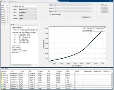
The curve fitting tool image shown below is godness-of-fit parameters are displayed for the different order ploynomial equations for the same data and compared which will be the best fit .

Code to fit a linear and cubic polynomial equation for the Cp data:

clear all
close all
clc
 %preparing the data
 Cp_data=load('data');
 temperature=Cp_data(:,1);
 Cp=Cp_data(:,2);
 
 
%Linear fit
%Cp=a*T+b
co_effs1=polyfit(temperature,Cp,1)
predicted_Cp1=polyval(co_effs1,temperature);
 
%curve fit
%Cp=a*T^3+b*T^2+C*T+D
co_effs=polyfit(temperature,Cp,3)
predicted_Cp3=polyval(co_effs,temperature);
 
%compare cubic curve fit with the original data
figure(1)
plot(temperature,Cp,'linewidth',3)
hold on
plot(temperature,predicted_Cp3,'linewidth',3,'color','r')
 xlabel('Temperature[K]')
ylabel('Specific Heat[kj/mol-k]')
legend('Original Dataset','Cubic Curve Fit')
 
%compare Linear curve fit with the original data
figure(2)
plot(temperature,Cp,'linewidth',3)
hold on
plot(temperature,predicted_Cp1,'linewidth',3,'color','g')
xlabel('Temperature[K]')
ylabel('Specific Heat[kj/mol-k]')
legend('Original Dataset','Linear Curve Fit')

PLOT:

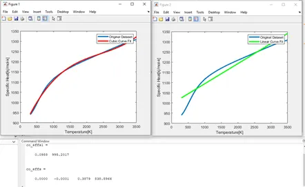
Plots for the Linear and cubic fit curves along with the raw data points. The results shows increasing the degree of polynimal equation the curve fits best to the Load data.

Evaluating using Curve Fitting Tool:

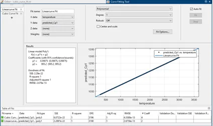
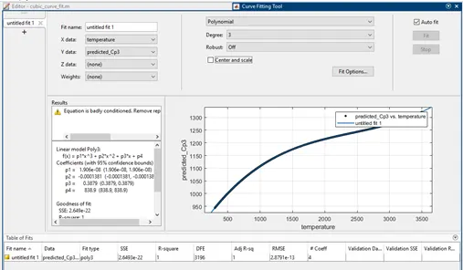
In the above image for cubic polynomial, throws a warning that the equation is badly conditioned. In that case it is better to evalute the perfect fit curve.

For large datasets, it is always better to split the data into eqaul fragments and perform fitting operation individually to determine the perfect fit.

Splitwise Method:

clear all
close all
clc

%variable n is length of data
Cp_data=load('data');
 n=length(Cp_data);
 
 s=300;
 a=1;
 b=n/s;


for i=1:s
  
temperature=Cp_data(a:b,1);
 Cp=Cp_data(a:b,2);
 

co_effs1=polyfit(temperature,Cp,3)
predicted_Cp=polyval(co_effs1,temperature);

plot(temperature,Cp,'linewidth',1)
hold on
plot(temperature,predicted_Cp,'linewidth',3,'color','y')

a=b;
b=b+n/s;
end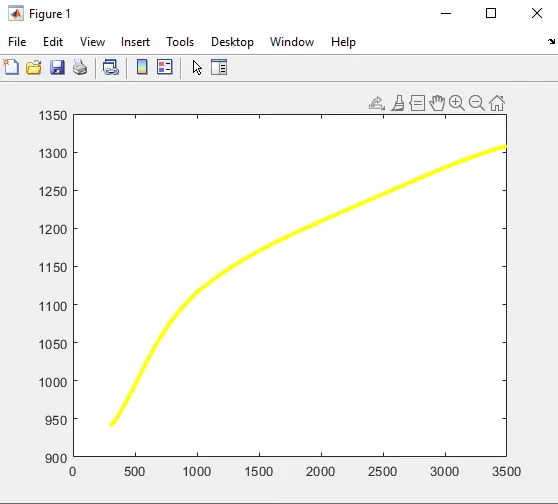

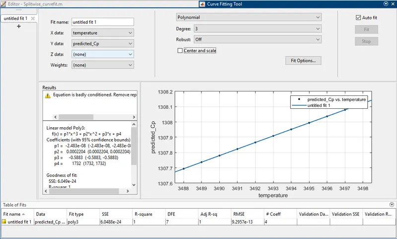
Even after doing splitting data method,we got the result that equation is badly conditioned. so we choose the linear curve is the best fit for the Load data.

Code to calculate the R2 value using Goodness-of-fit parameter to evaluate the best it.

clear all
close all
clc

Cp_data=load('data');
temperature=Cp_data(:,1);
cp=Cp_data(:,2);

co_effs=polyfit(temperature,cp,3);
predicted_cp=polyval(co_effs,temperature)

%error is difference between response value and precicted values of cp
error=cp-predicted_cp

% sse is sum ofsquares of errors
%initially assume sse=0
sse=0;
sum=0;
for i=1:length(cp)
sse=sse+error(i)^2;
sum=sum+cp(i);
end
n=length(cp)
mean=sum/n

%ssr is sum of squares of regression
ssr=0
for j=i:length(predicted_cp)
ssr=ssr+(predicted_cp(i)-mean)^2;
end
%calculating sst
sst=ssr+sse;
%r^2
r2=(ssr/sst)
%rmse,root mean square root
rmse=(sse/n)^0.5

% significant dependant variables added to equation which efffets the r2
% value.
k=2;

R_adj=1-((1-r2)*(n-1)/(n-k-1))

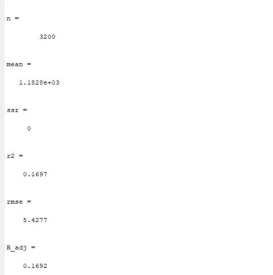
OUTPUT:

Confidence and Prediction bounds define the lower and upper values of the associated interval,and defines the width of the interval. A very wide interval for the fitted coefficients can indicate that we should use more data when fitting. The level of certainty is often 95%

Referrence:

https://skill-lync.com/projects/Curve-Fitting-and-criterion-to-choose-best-fit-41860

Conclusion:

We should examine all available goodness-of-fit measures before deciding on the which fit is best for the functionality of data. A graphical examination of the fit and residuals should always be initial approach. However, some fit characteristics are revealed only through numerical fit, results, statistics and predictions bounds.