Stability analysis in the unsteady state equation
# Unsteady state 2D Heat conduction equation.
Implicit form : the equation is given as follows :
`T_P^(n+1) = 1/(1+2*k1+2*k2)*[T_P^n + k1*(T_L+T_R)^(n+1) + k2*(T_T+T_B)^(n+1)]`
the code to simulate the results of the above equation is as follows :
% Unsteady state solver, implicit method.
clc
close all
clear all


L = 1;
t = 300;
nx = 20;
ny = 20;
alpha = 1.4;
dx = L/(nx-1);
dy = L/(ny-1);
dt = 1e-2;
%nt = t/dt;
nt = 1000
x = linspace(0,1,nx);
y = linspace(0,1,ny);
[xx,yy] = meshgrid(x,y);
k1 = alpha*dt/(dx^2);
k2 = alpha*dt/(dy^2);
CFL = k1+k2;


% initial and boundary conditions
T = 300*ones(nx);
T(1:ny,1) = 400;  %left
T(1,1:nx) = 600;  %top
T(ny,1:ny) = 900; %right
T(1:nx,nx) = 800; %bottom
% temperature at corners taken as the average of the adjacent walls
T(1,1) = 500;
T(1,nx) = 750;
T(ny,1) = 650;
T(nx,ny) = 850;
term1 = 1/(1+(2*k1)+(2*k2));
term2 = k1*term1;
term3 = k2*term1;
error = 9e9;
tol = 1e-4;
% initialize
Told = T;
Tprev = T;

% unsteady explicit
iterative_solver = 1    % the no. to this command can be changed to avail the required solver.

% Jacobi solver
if iterative_solver == 1
    jacobi_iter = 1;
   tic
 % time loop
 for m = 1:nt;
     error = 9e9;
     while error > tol
        %space loop
        for i = 2:nx-1
            for j = 2:ny-1
                T(i,j) = term1*Tprev(i,j) + term2*(Told(i-1,j)+Told(i+1,j)) + term3*(Told(i,j+1)+Told(i,j-1));
            end
        end
        error = max(max(abs(Told-T)));
        Told = T;
        jacobi_iter = jacobi_iter +1;
     end
     Tprev = T
end
jacobi_time = toc


    figure(1)
    contourf(xx,yy,T);
    colormap(jet);
    colorbar;
    xlabel('X-axis');
    ylabel('Y-axis');
    ax = gca;
    ax.YDir = 'reverse';
    title_text = sprintf('jacobi iteration no = %d',jacobi_iter);
    title_text1 = sprintf('jacobi time = %d',jacobi_time);
    title(title_text);
    title(title_text1,title_text);
end


%% G-S solver
if iterative_solver == 2
    gs_iter = 1;
   tic
 % time loop
 for m = 1:nt;
     error = 9e9;
     while error > tol
        %space loop
        for i = 2:nx-1
            for j = 2:ny-1
                T(i,j) = term1*Tprev(i,j) + term2*(T(i-1,j)+Told(i+1,j)) + term3*(T(i,j+1)+Told(i,j-1));
            end
        end
        error = max(max(abs(Told-T)));
        Told = T;
        gs_iter = gs_iter +1;
     end
     Tprev = T;
end
gs_time = toc

    figure(1)
    contourf(xx,yy,T);
    colormap(jet);
    colorbar;
    xlabel('X-axis');
    ylabel('Y-axis');
    ax = gca;
    ax.YDir = 'reverse';
    title_text = sprintf('GS iteration no = %d',gs_iter);
    title_text1 = sprintf('GS time = %d',gs_time);
    title(title_text,title_text1);
end


%% SOR method solver

if iterative_solver == 3

 w = 1.2
 sor_iter = 1
 tic
 for m = 1:nt;
     error = 9e9;
     tol = 1e-4;
    while error > tol;

    for i = 2:nx-1
        for j = 2:ny-1
            T(i,j) = term1*Tprev(i,j) + term2*(T(i-1,j)+Told(i+1,j)) + term3*(T(i,j+1)+Told(i,j-1));
            T(i,j) = ((1-w)*Told(i,j)) + (w*T(i,j));
        end
    end
    error = max(max(abs(Told - T)))
    Told = T;
    M(sor_iter)=getframe(gcf);
    sor_iter = sor_iter + 1;


    end
    Tprev = T;


 end
sor_time = toc;

    figure(1)
    contourf(xx,yy,T);
    colormap(jet)
    colorbar
    xlabel('X-axis')
    ylabel('Y-axis')


    title_text = sprintf('sor iteration no = %d',sor_iter);
    title_text1 = sprintf('SOR time = %d',sor_time);
    title(title_text,title_text1);
    ax = gca;
    ax.YDir = 'reverse';
    grid on
end


%      movie(M)
%      videofile = VideoWriter('Unsteady Implicit SOR.avi','Uncompressed AVI');
%      open(videofile)
%      writeVideo(videofile,M)
%      close(videofile)


%bar graph for iteration comparison
% steady_sor = 143
% unsteady_sor = 4592
% iteration = [steady_sor,unsteady_sor]
% figure(3)
% bar(iteration,0.40,'green')
% xticklabels({'steady-sor','unsteady-sor'})
% title('iteration comparison')
the results are as follows :
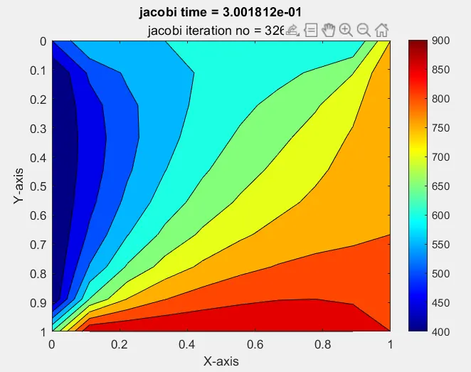
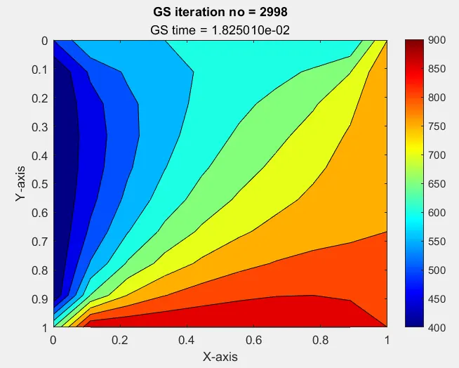
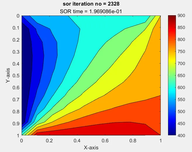
Since in Unsteady implicit case , the solution is independent of the variance in value of dt. Hence the CFL condition of (CFL less than and equal to 0.5)
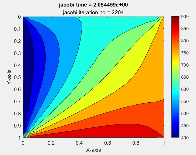
is not contributing towards the stability of the solution.
here is the graph of jacobi method with dt = 20. The CFL no. goes way beyond 0.5 value , yet we can see the solution is no blowing up.
# Unsteady state - Explicit form
the formula is given as : `T_P^(n+1) = 1/(1+2*k1+2*k2)*[T_P^n + k1*(T_L+T_R) + k2*(T_T+T_B)]^(n)`
the code :
% UNSTEADY 2D HEAT CONDUCTION USING EXPLICIT METHOD

clc
close all
clear all

L = 1;
t = 1000;
nx = 10;
ny = 10;
alpha = 1.4;
dx = L/(nx-1);
dy = L/(ny-1);
%dt = 0.00295
dt = 0.0023015%1e-3 % %0.0023015 1e-3
%nt = t/dt;
nt = 1500
x = linspace(0,1,nx);
y = linspace(0,1,ny);
[xx,yy] = meshgrid(x,y);
k1 = alpha*dt/(dx^2);
k2 = alpha*dt/(dy^2);
CFL = k1+k2;
iterative_solver = 1

% initial and boundary conditions
T = 300*ones(nx);
T(1:ny,1) = 400;  %left
T(1,1:nx) = 600;  %top
T(ny,1:ny) = 900; %right
T(1:nx,nx) = 800; %bottom
% temperature at corners taken as the average of the adjacent walls
T(1,1) = 500;
T(1,nx) = 750;
T(ny,1) = 650;
T(nx,ny) = 850;

% initialize
Told = T;

% unsteady explicit
if iterative_solver == 1
   iter = 1
 % time loop
 tic
for m = 1:nt;

    % space loop
    for i = 2:nx-1;
        for j = 2:ny-1;
            T(i,j) = Told(i,j) + (k1*(Told(i-1,j) - 2*Told(i,j) + Told(i+1,j))) + (k2*(Told(i,j+1) - 2*Told(i,j) + Told(i,j-1)));
        end
    end

    %error = max(max(abs(Told - T)));
    Told = T;
    iter = iter + 1

end

end

explicit_time = toc

figure(1)
contourf(xx,yy,T);
colormap(jet);
colorbar;
xlabel('X-axis');
ylabel('Y-axis');
ax = gca;
ax.YDir = 'reverse';
%title_text = sprintf('iteration no = %d',iter)
title_text1 = sprintf('explicit_time = %d',explicit_time)
title_text2 = sprintf('time step = %d',dt)
title(title_text1,title_text2)


% bar graph for iteration comparison
% iteration = [jacobi_iter,gs_iter,sor_iter]
% figure(3)
% bar(iteration,0.40,'green')
% xticklabels({'jacobi_iter','gs_iter','sor_iter'})
% title('iteration comparison')
In the code we change the value of dt and observe the changes in the solution.
Here the variation in the dt varies the stability of the solution. the formula for CFL is given as
CFL = k1 + k2 ; where, `k1 = alpha*(delt)/(delx^2) and k2 = alpha*(delt)/(dely^2)`
when `CFL le 0.5` then the solution is more likely to converge towards the stability. CFL is directly proportional to the dt.
Hence increase in dt more than a certain value will lead to increase in CFL more than 0.5 and will lead to blow up of the solution.
Unstablity in equation is not good for the CFD applications as the results are un-physical.
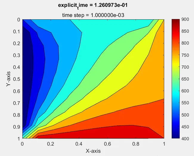
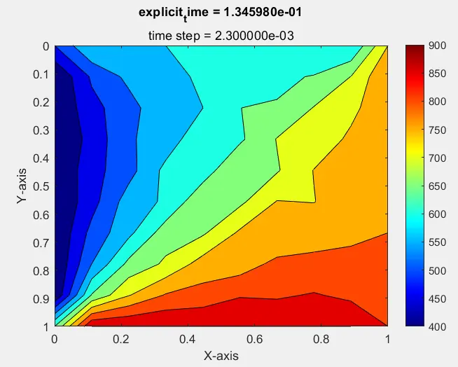
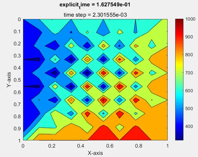
the results for various values for dt is given as follow :
the dt values are specified in the title of the graphs.
 ===>
===> 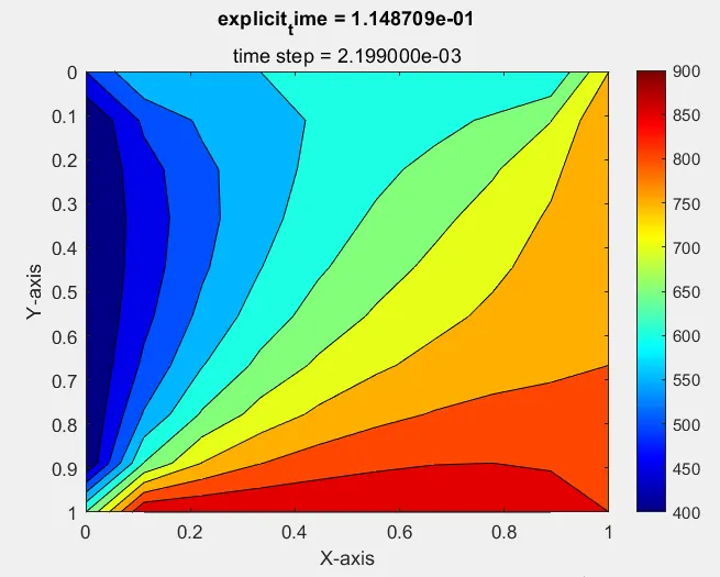
the above graphs are when CFL = 0.5216, the solution would have started to blow up when it went above 0.5 but the no. of grid points at which the solution is solved is less, hence the graph is not able to reflect the changes it went through when the solution blowed up at CFL >0.5.
 ===>
===> 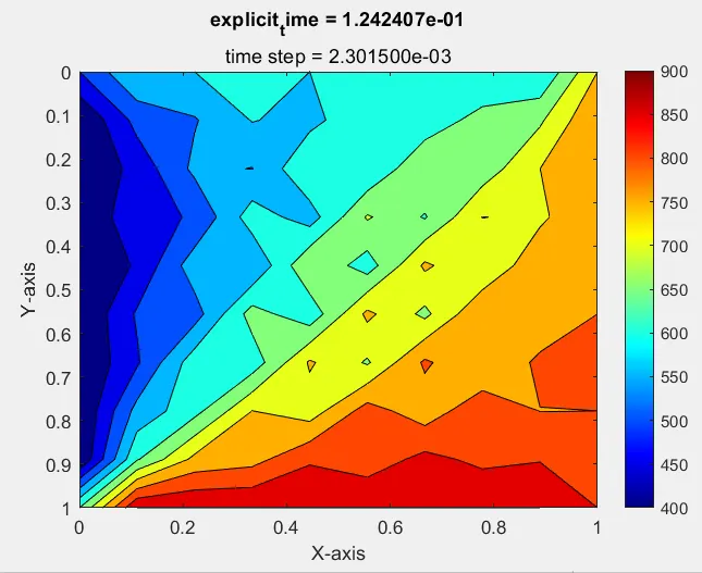
here in above graphs , the CFL = 0.5220. the solution has started to show clearly that is blowing up.
 ===>
===> 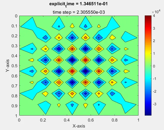
Here in above graphs, a complete blow up of solution is visible.
=============================== End ===================================