Stability analysis in the unsteady problem
AIM: For both implicit and explicit methods look at the effect of time step on the stability of the solution.
1.To observe how does an unstable solution look like?
2. At what CFL number does the solution become unstable ?
TRANSIENT CASE:
There two methods used in the transient case,
- Implicit method
- Explicit method
In the explicit method the iterative techniques are not used since all the values are known, But in the case of implicit method all the values are not known so the iterative techniques are used namely,
- Jacobi method
- Gauss seidal method
- SOR method
EXPLICIT METHOD:
The explicit is a direct method which is solved using the known values, The CFL number plays a vital role in the explicit form. For the above case the CFL number should be less than 0.5.
The normal CFL number for a numerical equation is,
`C = c frac{Deltat}{Deltax}le 1`
Where C is called the courant number
The equation says that `Deltatle frac{Deltax}{c}` for an numerical equation. This is called as the COURANT-FRIEDRICHS-LEWY condition
The CFL condition for the 2D dimensional heat conduction problem is
`alpha(frac{Deltat}{(Deltax)^2} + frac{Deltat}{(Deltay)^2}) le 0.5`
The above analysis method is called VON NEUMANN STABILITY METHOD
As long as CFL number remains below 0.5 the solution stays stable, if it reaches above 0.5 the solution becomes unstable.
Obsevation of effect on time steps in the stability of the solution:
The below code is nt = 800 and Time step dt = 1/5000, Where the CFL number is 0.3700 which is lesser than 0.5 so the solution becomes unstable.
MATLAB CODE FOR EXPLICIT METHOD:
clear all
close all
clc

nx = 30;
ny = nx;

x = linspace(0,1,nx);
y = linspace(0,1,ny);

dx = x(2) - x(1);
dy = y(2) - y(1);


omega = 1.1;
tol = 1e-4;
dt =1/5000;

T_L = 400;
T_T = 600;
T_R = 800;
T_B = 900;
T = ones(nx,ny);

T(2:ny-1,1) = T_L;
T(2:ny-1,nx) = T_R;
T(1,2:nx-1) = T_T;
T(nx,2:ny-1) = T_B;

T(1,1) = (T_T + T_L)/2;
T(nx,ny) = (T_R + T_B)/2;
T(1,ny) = (T_T + T_R)/2;
T(nx,1) = (T_B + T_L)/2;

k1 = (omega*dt)/(dx^2);
k2 = (omega*dt)/(dy^2);
nt = 800;
cfl = omega*(1/(dx^2) + 1/(dy^2))*(dt);

[X,Y] = meshgrid(x,y);
told = T;


    tic;
         for g = 1:nt

            for i = 2:nx-1
                for j = 2:ny-1
                    term1 = told(i,j);
                    term2 = k1*(told(i+1,j) - 2*told(i,j) + told(i-1,j));
                    term3 = k2*(told(i,j+1) - 2*told(i,j) + told(i,j-1));
                    T(i,j) = (term1 + term2 + term3);
                end
                end
                told = T;
            end


 f = toc;

 [M,N] = contourf(X,Y,T);
 clabel(M,N)
 colormap(jet)
 colorbar
 title_text = sprintf('Total iterations = %d time taken = %fs',nt,f);
 title(title_text)
 xlabel('x axis')
 ylabel('y axix')
 set(gca,'ydir','reverse')
OUTPUT:
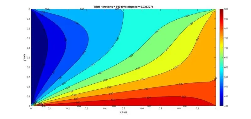
The above Plot shows that the system is stable. The above code is nt = 800 and Time step dt = 1/5000, Where the CFL number is 0.3700 which is lesser than 0.5 so the solution becomes stable.
The below code is for nt = 800 and the time step dt = 1/3000, Where the CFL number becomes 0.6167 which is greater than 0.5 so the solution becomes unstable.
MATLAB CODE FOR EXPLICIT METHOD:
clear all
close all
clc

nx = 30;
ny = nx;

x = linspace(0,1,nx);
y = linspace(0,1,ny);

dx = x(2) - x(1);
dy = y(2) - y(1);


omega = 1.1;
tol = 1e-4;
dt =1/3000;

T_L = 400;
T_T = 600;
T_R = 800;
T_B = 900;
T = ones(nx,ny);

T(2:ny-1,1) = T_L;
T(2:ny-1,nx) = T_R;
T(1,2:nx-1) = T_T;
T(nx,2:ny-1) = T_B;

T(1,1) = (T_T + T_L)/2;
T(nx,ny) = (T_R + T_B)/2;
T(1,ny) = (T_T + T_R)/2;
T(nx,1) = (T_B + T_L)/2;

k1 = (omega*dt)/(dx^2);
k2 = (omega*dt)/(dy^2);
nt = 800;
cfl = omega*(1/(dx^2) + 1/(dy^2))*(dt);

[X,Y] = meshgrid(x,y);
told = T;


    tic;
         for g = 1:nt

            for i = 2:nx-1
                for j = 2:ny-1
                    term1 = told(i,j);
                    term2 = k1*(told(i+1,j) - 2*told(i,j) + told(i-1,j));
                    term3 = k2*(told(i,j+1) - 2*told(i,j) + told(i,j-1));
                    T(i,j) = (term1 + term2 + term3);
                end
                end
                told = T;
            end


 f = toc;

 [M,N] = contourf(X,Y,T);
 clabel(M,N)
 colormap autumn
 colorbar
 title_text = sprintf('Total iterations = %d time taken = %fs',nt,f);
 title(title_text)
 xlabel('x axis')
 ylabel('y axix')
 set(gca,'ydir','reverse')
OUTPUT:
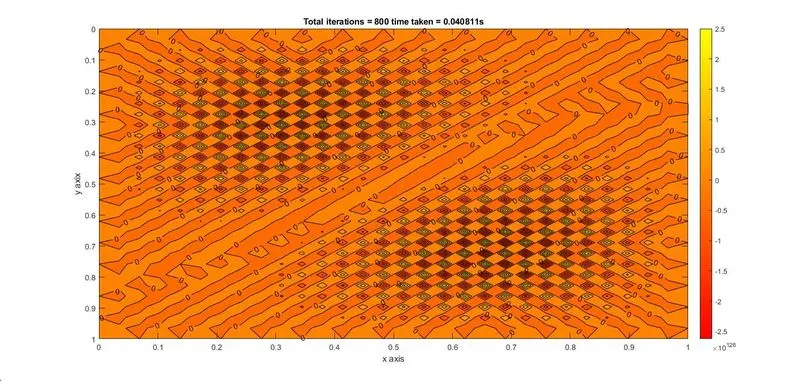
The above code is for nt = 800 and the time step dt = 1/3000, Where the CFL number becomes 0.6167 which is greater than 0.5 so the solution becomes unstable.
The above image depicts that the system is unstable. This because of decrease in the timestep dt. This clearly shows that the decrease in time step increases the CFL number which makes the solution unstable.
By the above analysis the sysytem goes unstable at CFL number 0.6167. So when its below this value the system achieves stable solution.
IMPLICIT METHOD:
There are three methods in the implicit method,
- Jacobi method
- Gauss seidal method
- SOR method
We all know that the implicit method is unconditionally stable, When the time step is increased still the solution is stable in implicit method.
The below code is a stable solution of the implicit method with nt = 800 and dt = 1/5000
and the CFL number is 0.3700
clear all
close all
clc


L = 1;
nx = 30;
ny = nx;

x = linspace(0,L,nx);
y = linspace(0,L,ny);

dx = x(2) - x(1);
dy = y(2) - y(1);


tol = 1e-4;
alpha = 1.4;


T_L = 400;
T_T = 600;
T_R = 800;
T_B = 900;
T = ones(nx,ny);

T(2:ny-1,1) = T_L;
T(2:ny-1,nx) = T_R;
T(1,2:nx-1) = T_T;
T(nx,2:ny-1) = T_B;

T(1,1) = (T_T + T_L)/2;
T(nx,ny) = (T_R + T_B)/2;
T(1,ny) = (T_T + T_R)/2;
T(nx,1) = (T_B + T_L)/2;
dt = 1/5000;
cfl = alpha*(1/(dx^2) + 1/(dy^2))*(dt);
k1 = (alpha*dt)/(dx^2);
k2 = (alpha*dt)/(dy^2);
nt = 800;


[X,Y] = meshgrid(x,y);
told = T;
t_prev = told;

 iterative_solver =  1:3;
 for iterative_solver = 1
    tic;
    if iterative_solver == 1
        jacobi_iter = 1;
         for g = 1:nt
             error = 9e9;
        while(error > tol)
            for i = 2:nx-1
                for j = 2:ny-1
                     term1 = (1+(2*k1)+(2*k2))^-1;
                     term2 = k1*term1;
                     term3 = k2*term1;
                    H = told(i-1,j) + told(i+1,j);
                    V = told(i,j-1) + told(i,j+1);
                    T(i,j) = (t_prev(i,j)*term1) + (H*term2) + (V*term3);

                end
            end
            error = max(max(abs(told - T)));
            told = T;
            jacobi_iter = jacobi_iter + 1;
        end
        t_prev = T;
         end
    end

     f = toc;

 figure(1)
 subplot(2,2,1)
 [M,N] = contourf(X,Y,T);
 clabel(M,N)
 colormap(jet)
 colorbar
 title_text = sprintf('Total iterations(Jacobi) = %d  Simulation time = %fs',jacobi_iter,f);
 title(title_text)
 xlabel('x axis')
 ylabel('y axix')
 set(gca,'ydir','reverse')

 end


 L = 1;
nx = 30;
ny = nx;

x = linspace(0,L,nx);
y = linspace(0,L,ny);

dx = x(2) - x(1);
dy = y(2) - y(1);


tol = 1e-4;
alpha = 1.4;
dt = 1/5000;

T_L = 400;
T_T = 600;
T_R = 800;
T_B = 900;
T = ones(nx,ny);

T(2:ny-1,1) = T_L;
T(2:ny-1,nx) = T_R;
T(1,2:nx-1) = T_T;
T(nx,2:ny-1) = T_B;

T(1,1) = (T_T + T_L)/2;
T(nx,ny) = (T_R + T_B)/2;
T(1,ny) = (T_T + T_R)/2;
T(nx,1) = (T_B + T_L)/2;

cfl = alpha*(1/(dx^2) + 1/(dy^2))*(dt);
k1 = (alpha*dt)/(dx^2);
k2 = (alpha*dt)/(dy^2);
nt = 800;

    for iterative_solver = 2
  tic;
    if iterative_solver == 2
         gs_iter = 1;
         for g = 1:nt
             error = 9e9;
        while(error > tol)
            for i = 2:nx-1
                for j = 2:ny-1
                     term1 = (1+(2*k1)+(2*k2))^-1;
                     term2 = k1*term1;
                     term3 = k2*term1;
                    H = T(i-1,j) + told(i+1,j);
                    V = T(i,j-1) + told(i,j+1);
                    T(i,j) = (t_prev(i,j)*term1) + (H*term2) + (V*term3);

                end
            end
            error = max(max(abs(told - T)));
            told = T;
            gs_iter = gs_iter +  1;
        end
        t_prev = T;
         end
    end

 f2 = toc;

 figure(1)
 subplot(2,2,2)
 [M,N] = contourf(X,Y,T);
 clabel(M,N)
 colormap(jet)
 colorbar
 title_text = sprintf('Total iterations(gs) = %d  Simulation time = %fs',gs_iter,f2);
 title(title_text)
 xlabel('x axis')
 ylabel('y axix')
 set(gca,'ydir','reverse')


    end

 L = 1;
nx = 30;
ny = nx;

x = linspace(0,L,nx);
y = linspace(0,L,ny);

dx = x(2) - x(1);
dy = y(2) - y(1);


tol = 1e-4;
alpha = 1.4;
omega = 1.5;
dt = 1/5000;

T_L = 400;
T_T = 600;
T_R = 800;
T_B = 900;
T = ones(nx,ny);

T(2:ny-1,1) = T_L;
T(2:ny-1,nx) = T_R;
T(1,2:nx-1) = T_T;
T(nx,2:ny-1) = T_B;

T(1,1) = (T_T + T_L)/2;
T(nx,ny) = (T_R + T_B)/2;
T(1,ny) = (T_T + T_R)/2;
T(nx,1) = (T_B + T_L)/2;

cfl = alpha*(1/(dx^2) + 1/(dy^2))*(dt);
k1 = (alpha*dt)/(dx^2);
k2 = (alpha*dt)/(dy^2);
nt = 800;
for iterative_solver = 3
    omega = 1.4;
    tic;
    if iterative_solver == 3
        sor_iter = 1;
         for g = 1:nt
             error = 9e9;
        while(error > tol)
            for i = 2:nx-1
                for j = 2:ny-1
                     term1 = (1+(2*k1)+(2*k2))^-1;
                     term2 = k1*term1;
                     term3 = k2*term1;
                    H = T(i-1,j) + told(i+1,j);
                    V = T(i,j-1) + told(i,j+1);
                    T(i,j) = ((1-omega)*told(i,j)) + omega*((t_prev(i,j)*term1) + (H*term2) + (V*term3));

                end
            end
            error = max(max(abs(told - T)));
            told = T;
            sor_iter = sor_iter + 1;
        end
        t_prev = T;
         end
    end

 f3 = toc;

 figure(1)
 subplot(2,2,3)
 [M,N] = contourf(X,Y,T);
 clabel(M,N)
 colormap(jet)
 colorbar
 title_text = sprintf('Total iterations(sor) = %d   Simulation time = %fs',sor_iter,f3);
 title(title_text)
 xlabel('x axis')
 ylabel('y axix')
set(gca,'ydir','reverse')

end
OUTPUT:
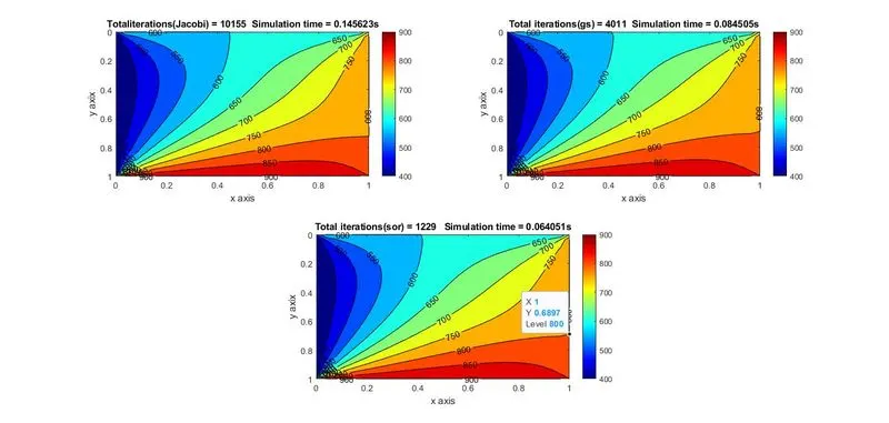
The above code states that the solution is stable.
The main advantage of the implicit method is that it is unconditionally stable. The effect of time step does not affect the solution.when the time step is increased also the solution is stable.
The below code is with increased time step of dt = 1/100
clear all
close all
clc


L = 1;
nx = 30;
ny = nx;

x = linspace(0,L,nx);
y = linspace(0,L,ny);

dx = x(2) - x(1);
dy = y(2) - y(1);


tol = 1e-4;
alpha = 1.4;


T_L = 400;
T_T = 600;
T_R = 800;
T_B = 900;
T = ones(nx,ny);

T(2:ny-1,1) = T_L;
T(2:ny-1,nx) = T_R;
T(1,2:nx-1) = T_T;
T(nx,2:ny-1) = T_B;

T(1,1) = (T_T + T_L)/2;
T(nx,ny) = (T_R + T_B)/2;
T(1,ny) = (T_T + T_R)/2;
T(nx,1) = (T_B + T_L)/2;
dt = 1/100;
cfl = alpha*(1/(dx^2) + 1/(dy^2))*(dt);
k1 = (alpha*dt)/(dx^2);
k2 = (alpha*dt)/(dy^2);
nt = 800;


[X,Y] = meshgrid(x,y);
told = T;
t_prev = told;

 iterative_solver =  1:3;
 for iterative_solver = 1
    tic;
    if iterative_solver == 1
        jacobi_iter = 1;
         for g = 1:nt
             error = 9e9;
        while(error > tol)
            for i = 2:nx-1
                for j = 2:ny-1
                     term1 = (1+(2*k1)+(2*k2))^-1;
                     term2 = k1*term1;
                     term3 = k2*term1;
                    H = told(i-1,j) + told(i+1,j);
                    V = told(i,j-1) + told(i,j+1);
                    T(i,j) = (t_prev(i,j)*term1) + (H*term2) + (V*term3);

                end
            end
            error = max(max(abs(told - T)));
            told = T;
            jacobi_iter = jacobi_iter + 1;
        end
        t_prev = T;
         end
    end

     f = toc;

 figure(1)
 subplot(2,2,1)
 [M,N] = contourf(X,Y,T);
 clabel(M,N)
 colormap(jet)
 colorbar
 title_text = sprintf('Total iterations(Jacobi) = %d  Simulation time = %fs',jacobi_iter,f);
 title(title_text)
 xlabel('x axis')
 ylabel('y axix')
 set(gca,'ydir','reverse')

 end


 L = 1;
nx = 30;
ny = nx;

x = linspace(0,L,nx);
y = linspace(0,L,ny);

dx = x(2) - x(1);
dy = y(2) - y(1);


tol = 1e-4;
alpha = 1.4;
dt = 1/100;

T_L = 400;
T_T = 600;
T_R = 800;
T_B = 900;
T = ones(nx,ny);

T(2:ny-1,1) = T_L;
T(2:ny-1,nx) = T_R;
T(1,2:nx-1) = T_T;
T(nx,2:ny-1) = T_B;

T(1,1) = (T_T + T_L)/2;
T(nx,ny) = (T_R + T_B)/2;
T(1,ny) = (T_T + T_R)/2;
T(nx,1) = (T_B + T_L)/2;

cfl = alpha*(1/(dx^2) + 1/(dy^2))*(dt);
k1 = (alpha*dt)/(dx^2);
k2 = (alpha*dt)/(dy^2);
nt = 800;

    for iterative_solver = 2
  tic;
    if iterative_solver == 2
         gs_iter = 1;
         for g = 1:nt
             error = 9e9;
        while(error > tol)
            for i = 2:nx-1
                for j = 2:ny-1
                     term1 = (1+(2*k1)+(2*k2))^-1;
                     term2 = k1*term1;
                     term3 = k2*term1;
                    H = T(i-1,j) + told(i+1,j);
                    V = T(i,j-1) + told(i,j+1);
                    T(i,j) = (t_prev(i,j)*term1) + (H*term2) + (V*term3);

                end
            end
            error = max(max(abs(told - T)));
            told = T;
            gs_iter = gs_iter +  1;
        end
        t_prev = T;
         end
    end

 f2 = toc;

 figure(1)
 subplot(2,2,2)
 [M,N] = contourf(X,Y,T);
 clabel(M,N)
 colormap(jet)
 colorbar
 title_text = sprintf('Total iterations(gs) = %d  Simulation time = %fs',gs_iter,f2);
 title(title_text)
 xlabel('x axis')
 ylabel('y axix')
 set(gca,'ydir','reverse')


    end

 L = 1;
nx = 30;
ny = nx;

x = linspace(0,L,nx);
y = linspace(0,L,ny);

dx = x(2) - x(1);
dy = y(2) - y(1);


tol = 1e-4;
alpha = 1.4;
omega = 1.5;
dt = 1/100;

T_L = 400;
T_T = 600;
T_R = 800;
T_B = 900;
T = ones(nx,ny);

T(2:ny-1,1) = T_L;
T(2:ny-1,nx) = T_R;
T(1,2:nx-1) = T_T;
T(nx,2:ny-1) = T_B;

T(1,1) = (T_T + T_L)/2;
T(nx,ny) = (T_R + T_B)/2;
T(1,ny) = (T_T + T_R)/2;
T(nx,1) = (T_B + T_L)/2;

cfl = alpha*(1/(dx^2) + 1/(dy^2))*(dt);
k1 = (alpha*dt)/(dx^2);
k2 = (alpha*dt)/(dy^2);
nt = 800;
for iterative_solver = 3
    omega = 1.4;
    tic;
    if iterative_solver == 3
        sor_iter = 1;
         for g = 1:nt
             error = 9e9;
        while(error > tol)
            for i = 2:nx-1
                for j = 2:ny-1
                     term1 = (1+(2*k1)+(2*k2))^-1;
                     term2 = k1*term1;
                     term3 = k2*term1;
                    H = T(i-1,j) + told(i+1,j);
                    V = T(i,j-1) + told(i,j+1);
                    T(i,j) = ((1-omega)*told(i,j)) + omega*((t_prev(i,j)*term1) + (H*term2) + (V*term3));

                end
            end
            error = max(max(abs(told - T)));
            told = T;
            sor_iter = sor_iter + 1;
        end
        t_prev = T;
         end
    end

 f3 = toc;

 figure(1)
 subplot(2,2,3)
 [M,N] = contourf(X,Y,T);
 clabel(M,N)
 colormap(jet)
 colorbar
 title_text = sprintf('Total iterations(sor) = %d   Simulation time = %fs',sor_iter,f3);
 title(title_text)
 xlabel('x axis')
 ylabel('y axix')
set(gca,'ydir','reverse')

end
OUTPUT:
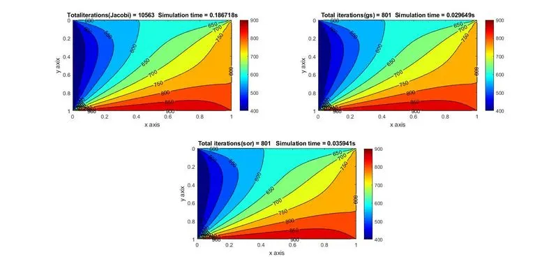
From the above outputs it is clear that increase in the time step does not make the solution unstable in implicit method likewise in the explicit method. That is the reason why implicit method is called unconditionally stable.
CONCLUSION:
In case explicit method the stability is highly dependent on the CFL number.
`alpha(frac{Deltat}{(Deltax)^2} + frac{Deltat}{(Deltay)^2}) le 0.5`
The CFL number should be less than 0.5.
When the CFL number is less than 0.5 the solution is stable.when it increases the system goes unstable as shown in above outputs.
The effect of time step is also plays an vital role here, As the time step increases the CFL number also gets increased which makes the solution unstable.
In case of the implicit method it is unconditionally stable so having more CFL number does not affect the stability of the solution. In implicit method higher time step can be used compared with explicit as the increase in the timestep does not affect the stability of the solution.
Overall to determine which method to be used whether it is explicit or implicit largely dependent upon the goals of computation. When time accuracy required explicit gives greater accuracy with less computational time.