Solving the steady and unsteady 2D heat conduction problem
Aim : Solve the 2D heat conduction equation by using the point iterative techniques.
Procedure : Let us consider a rectangular plate which is subjected to different temperature values at its boundaries. The heat conduction inside these boundaries need to be determined in graphical format.
The 2D heat conduction equation is given as : `(delT)/(delt) + alpha*((del^2T)/(delx^2) + (del^2T)/(dely^2)) = 0`
They can be classified into two forms : Steady and Unsteady state.
Steady state is given as : `(del^2T)/(delx^2) + (del^2T)/(dely^2) = 0` and unsteady as above equation.
If we discretize the equation of steady and unsteady state we get as follows :
Steady state : `T_p^n = 1/k[(T_L + T_R)/dx^2] + 1/k[(T_T + T_B)/dy^2]`
Unsteady state : `T_p^(n+1) = 1/(1+2k1+2k2)*[T_p^(n) + k1*(T_L+T_R)^(n+1) + k2*(T_T+T_B)^(n+1)`
where `k1 = alpha*(delt)/(delx^2) and k2 = alpha*(delt)/(dely^2)` and
`T_T = T(i,j+1) , T_B = T(i,j-1) , T_L = T(i-1,j) , T_R = T(i+1,j)`
The boundary conditions are specified as :
Top Boundary = 600 K
Bottom Boundary = 900 K
Left Boundary = 400 K
Right Boundary = 800 K
Let us divide the domain in discrete points as node and specify initially the temperature inside these boundaries as 300 K.
Coding walkthrough :
After defining the initial and boundary conditions as above, the solve the steady state equation by Jacobi , Gauss Seidal and Successive over-relaxation method. The code is as follows :
For Jacobi method : the T values taken will be the old values of temperatures with the space loop.
For Gauss Seidal method : we take the new values of T as we solve the equation.
For SOR method : we use the formula as : `T(i,j) = (1-w)*T_(old) + w*(T_(GS))`
T_(GS) = T calculated by Gauss Seidal method. Note: `w > 1 (over-relaxation) and w < 1 then (under-relaxation)`
the code is as follows :
### Steady state
clear all
close all
clc

L = 1;
nx = 10;
ny = 10;
dx = L/(nx-1);
dy = L/(ny-1);
dt = 1e-2;
x = linspace(0,1,nx);
y = linspace(0,1,ny);
[xx,yy] = meshgrid(x,y)
%zz = [xx,yy]
% initial and boundary conditions
T = 300*ones(nx);
T(1:ny,1) = 400;  %left
T(1,1:nx) = 600;  %top
T(ny,1:ny) = 900; %right
T(1:nx,nx) = 800; %bottom
T(1,1) = 500;
T(1,nx) = 750;
T(ny,1) = 650;
T(nx,ny) = 850;

Told = T
k = 2*(((dx)^2+(dy)^2)/((dx^2)*(dy^2)));
% steady state 2D heat conduction
% Explicit
% Jacobi
error = 1;
tol = 1e-4
iterative_solver = 1

% code for jacobi iterative solver

if iterative_solver == 1
   jacobi_iter = 1
    while error > tol;
    for i = 2:nx-1
        for j = 2:ny-1
            %[T(i,j)] = steady_explicit(dx(i),dy(j),k,Told)
            term1 = 1/k*((Told(i-1,j) + Told(i+1,j))/(dx^2));
            term2 = 1/k*((Told(i,j+1)+Told(i,j-1))/(dy^2));
            T(i,j) = term1 + term2;
        end
    end
    error = max(max(abs(Told - T)));
    Told = T;
    jacobi_iter = jacobi_iter + 1


    end


    figure(1)
    contourf(xx,yy,T);
    colormap(jet)
    colorbar
    xlabel('X-axis')
    ylabel('Y-axis')
    ax = gca;
    ax.YDir = 'reverse';
    title_text = sprintf('Jacobi iteration no = %d',jacobi_iter);
    title(title_text);
end


%% code for gauss seidel solver
if iterative_solver == 2
    gs_iter = 1
    while error > tol;
    for i = 2:nx-1
        for j = 2:ny-1
            %[T(i,j)] = steady_explicit(dx(i),dy(j),k,Told)
            term1 = 1/k*((T(i-1,j) + Told(i+1,j))/(dx^2));
            term2 = 1/k*((T(i,j+1)+Told(i,j-1))/(dy^2));
            T(i,j) = term1 + term2;
        end
    end
    error = max(max(abs(Told - T)))
    Told = T;
    gs_iter = gs_iter + 1


    end

    figure(2)
    contourf(xx,yy,T);
    colormap(jet)
    colorbar
    xlabel('X-axis')
    ylabel('Y-axis')
    ax = gca;
    ax.YDir = 'reverse';

    title_text = sprintf('Gauss Seidel iteration no = %d',gs_iter);
    title(title_text);
end


%% SOR approach

if iterative_solver == 3

 w = 1.1
 sor_iter = 1
    while error > tol;
    for i = 2:nx-1
        for j = 2:ny-1
            term1 = 1/k*((T(i-1,j) + Told(i+1,j))/(dx^2));
            term2 = 1/k*((T(i,j+1)+Told(i,j-1))/(dy^2));
            T(i,j) = term1 + term2;
            T(i,j) = ((1-w)*Told(i,j)) + (w*T(i,j));
        end
    end
    error = max(max(abs(Told - T)))
    Told = T;
    sor_iter = sor_iter + 1


    end

    figure(3)
    contourf(xx,yy,T);
    colormap(jet)
    colorbar
    xlabel('X-axis')
    ylabel('Y-axis')

    title_text = sprintf('sor iteration no = %d',sor_iter);
    title(title_text);
    ax = gca;
    ax.YDir = 'reverse';
end
we can change the number for iterative solver from 1 to 3 and avail the results for all the methods.
as we progress through various methods of iterative solvers we see that different methods converge the results in different no. of iterations.
result for jacobi method :
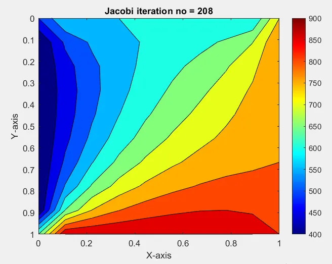
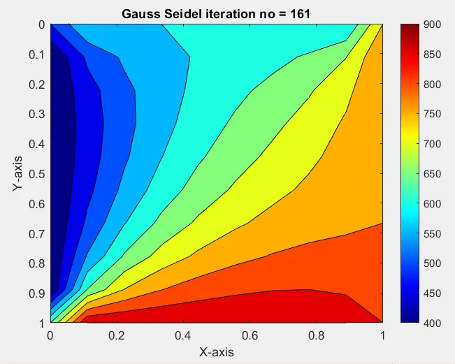
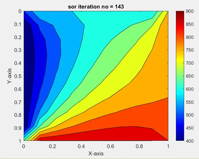
As we can see from the above graphs , the sor iteration method shows a converged result in lesser no. of iterations.
Let us look at the Unsteady state of 2D Heat conduction equation. Here we use Explicit and Implicit method to solve it.
It has time derivative term hence we use these both methods.
The formula for explicit form is given as : `T_P^(n+1) = T_P^n + k1*(T_L-2*T_P+T_R)^n + k2*(T_T-2*T_P+T_B)^n`
where, `k1 = alpha*(delt)/(delx) and k2 = alpha*(delt)/(dely)` and CFL = k1+k2. The CFL is a stability criteria where it determines the convergence of the equation. The CFL no. should be less than or equal to 0.5.
and alpha should be checked against 1.4 or 1.5 to see the variation in equation.
The code is given as follows :
### Unsteady state
% UNSTEADY 2D HEAT CONDUCTION USING EXPLICIT METHOD

clc
close all
clear all

L = 1;
t = 1000;
nx = 10;
ny = 10;
alpha = 1.4;
dx = L/(nx-1);
dy = L/(ny-1);
dt = 1e-3
%nt = t/dt;
nt = 1000
x = linspace(0,1,nx);
y = linspace(0,1,ny);
[xx,yy] = meshgrid(x,y);
k1 = alpha*dt/(dx^2);
k2 = alpha*dt/(dy^2);
iterative_solver = 1

% initial and boundary conditions
T = 300*ones(nx);
T(1:ny,1) = 400;  %left
T(1,1:nx) = 600;  %top
T(ny,1:ny) = 900; %right
T(1:nx,nx) = 800; %bottom
% temperature at corners taken as the average of the adjacent walls
T(1,1) = 500;
T(1,nx) = 750;
T(ny,1) = 650;
T(nx,ny) = 850;

% initialize
Told = T;

% unsteady explicit
if iterative_solver == 1
    iter = 1;

 tic
 % time loop
for m = 1:nt;
    % space loop
    for i = 2:nx-1;
        for j = 2:ny-1;
            T(i,j) = Told(i,j) + (k1*(Told(i-1,j) - 2*Told(i,j) + Told(i+1,j))) + (k2*(Told(i,j+1) - 2*Told(i,j) + Told(i,j-1)));

        end
    end

    %error = max(max(abs(Told - T)));
    Told = T;


    iter = iter + 1;
end
end
time = toc
    figure(1)
    contourf(xx,yy,T);
    colormap(jet);
    colorbar;
    xlabel('X-axis');
    ylabel('Y-axis');
    ax = gca;
    ax.YDir = 'reverse';
    title_text = sprintf('iteration no = %d',iter);
    title_text1 = sprintf('time = %d',time);
    title(title_text);
    title(title_text1);
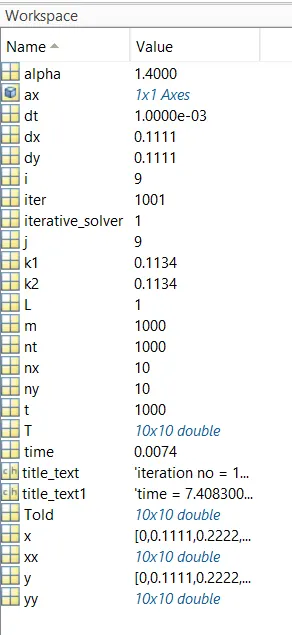
time taken for the solution is captured in the title of the plot. the results are given as follows :
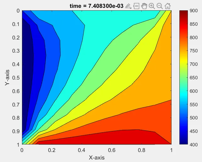
Unsteady state - Implicit method.
Here we will use iterative solvers to find the solution.
the fomula is given as : `T_P^(n+1) = 1/(1+2*k1+2*k2)*[T_P^n + k1*(T_L+T_R)^(n+1) + k2*(T_T+T_B)^(n+1)]`
where, `k1 = alpha*(delt)/(delx^2) and k2 = alpha*(delt)/(dely^2)`
In this method we use the Tprev value as T in the time loop and Told value as T in the space loop. Since we want to update the values of them as we progress through the loop.
the code is given as follows :
% Unsteady state solver, implicit method.

clc
close all
clear all

L = 1;
t = 1400;
nx = 10;
ny = 10;
alpha = 1.4;
dx = L/(nx-1);
dy = L/(ny-1);
dt = 1e-3;
%nt = t/dt;
nt = 1000
x = linspace(0,1,nx);
y = linspace(0,1,ny);
[xx,yy] = meshgrid(x,y);
k1 = alpha*dt/(dx^2);
k2 = alpha*dt/(dy^2);


% initial and boundary conditions
T = 300*ones(nx);
T(1:ny,1) = 400;  %left
T(1,1:nx) = 600;  %top
T(ny,1:ny) = 900; %right
T(1:nx,nx) = 800; %bottom
% temperature at corners taken as the average of the adjacent walls
T(1,1) = 500;
T(1,nx) = 750;
T(ny,1) = 650;
T(nx,ny) = 850;
term1 = 1/(1+(2*k1)+(2*k2));
term2 = k1*term1;
term3 = k2*term1;
error = 9e9;
tol = 1e-4;
% initialize
Told = T;
Tprev = T;

% unsteady explicit
iterative_solver = 1    % the no. to this command can be changed to avail the required solver.

% Jacobi solver
if iterative_solver == 1
    jacobi_iter = 1;
   tic
 % time loop
 for m = 1:nt;
     error = 9e9;
     while error > tol
        %space loop
        for i = 2:nx-1
            for j = 2:ny-1
                T(i,j) = term1*Tprev(i,j) + term2*(Told(i-1,j)+Told(i+1,j)) + term3*(Told(i,j+1)+Told(i,j-1));
            end
        end
        error = max(max(abs(Told-T)));
        Told = T;
        jacobi_iter = jacobi_iter +1;
     end
     Tprev = T
end
jacobi_time = toc


    figure(1)
    contourf(xx,yy,T);
    colormap(jet);
    colorbar;
    xlabel('X-axis');
    ylabel('Y-axis');
    ax = gca;
    ax.YDir = 'reverse';
    title_text = sprintf('jacobi iteration no = %d',jacobi_iter);
    title_text1 = sprintf('jacobi time = %d',jacobi_time);
    title(title_text);
    title(title_text1,title_text);
end


%% G-S solver
if iterative_solver == 2
    gs_iter = 1;
   tic
 % time loop
 for m = 1:nt;
     error = 9e9;
     while error > tol
        %space loop
        for i = 2:nx-1
            for j = 2:ny-1
                T(i,j) = term1*Tprev(i,j) + term2*(T(i-1,j)+Told(i+1,j)) + term3*(T(i,j+1)+Told(i,j-1));
            end
        end
        error = max(max(abs(Told-T)));
        Told = T;
        gs_iter = gs_iter +1;
     end
     Tprev = T;
end
gs_time = toc

    figure(2)
    contourf(xx,yy,T);
    colormap(jet);
    colorbar;
    xlabel('X-axis');
    ylabel('Y-axis');
    ax = gca;
    ax.YDir = 'reverse';
    title_text = sprintf('GS iteration no = %d',gs_iter);
    title_text1 = sprintf('GS time = %d',gs_time);
    title(title_text,title_text1);
end


%% SOR method solver

if iterative_solver == 3

 w = 1.2
 sor_iter = 1
 tic
 for m = 1:nt;
     error = 9e9;
     tol = 1e-4;
    while error > tol;

    for i = 2:nx-1
        for j = 2:ny-1
            T(i,j) = term1*Tprev(i,j) + term2*(T(i-1,j)+Told(i+1,j)) + term3*(T(i,j+1)+Told(i,j-1));
            T(i,j) = ((1-w)*Told(i,j)) + (w*T(i,j));
        end
    end
    error = max(max(abs(Told - T)))
    Told = T;
    sor_iter = sor_iter + 1;

    end
    Tprev = T;

 end
 sor_time = toc

    figure(3)
    contourf(xx,yy,T);
    colormap(jet)
    colorbar
    xlabel('X-axis')
    ylabel('Y-axis')
    title_text = sprintf('sor iteration no = %d',sor_iter);
    title_text1 = sprintf('SOR time = %d',sor_time);
    title(title_text,title_text1);
    ax = gca;
    ax.YDir = 'reverse';
end
the result is given as follows :
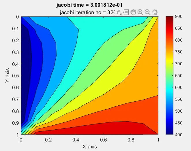
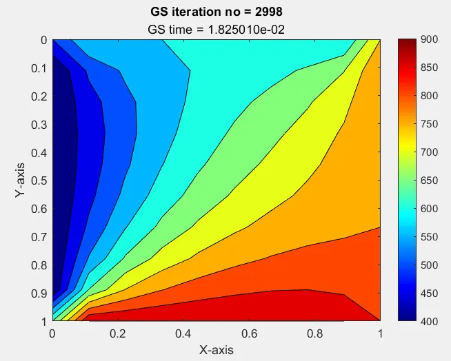
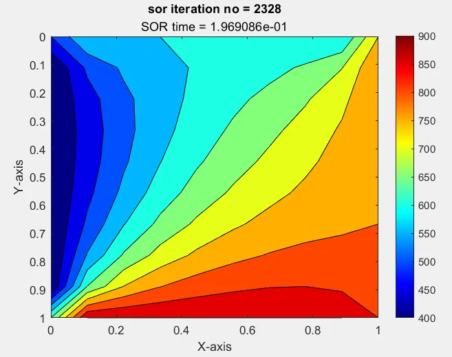
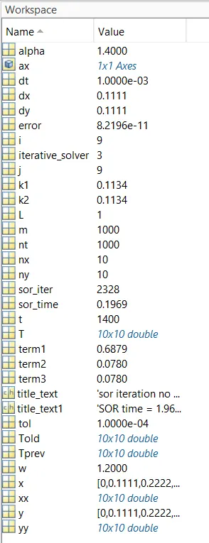
As we can see the lesser no. of iterations taken by sor, it is effective to solve the equation and converge the solution at a faster rate.
the animation video link for the convergence for the SOR method in Implicit Unsteady state is given as follows:
================================ End =====================================