Solving Second Order ODE's using MATLAB

Aim: To solve scond order ODE's in

Objective: To solve the given second order ODE of a simple pendulum with damping and plot the results on MATLAB

Theory:

A simple pendulum consists of a mass suspended at the end of a string wire with zero or negligeble mass. If the pendulum wieght is pulled to a side at a relatively small angle, the pendulum will keep moving back and forth at a regular period and frequency.

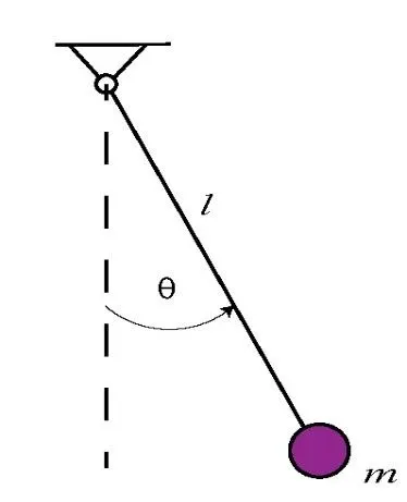
The movement of the pendulum can be described using the second order ODE below

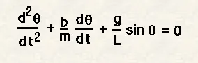
where,

b = damping co-efficient

m = mass of the weight suspended in Kg

g = gravitational force in m/s^2

L = length of the string in m

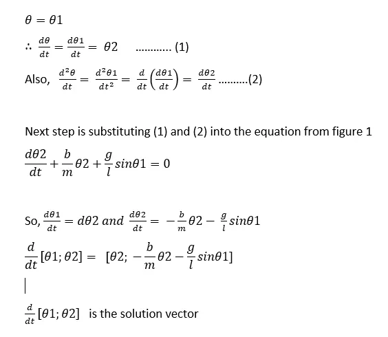
By breaking down the given second order ODE into 2 first order ODE's we get the following results

Code:

Fuction Definition:

function [dtheta_dt] = ode_func(t,theta,b,g,l,m)

theta1 = theta(1)
theta2 = theta(2)
dtheta1_dt = theta2;
dtheta2_dt = -(b/m)*theta2 - (g/l)*sin(theta1);
dtheta_dt = [dtheta1_dt; dtheta2_dt];
end

Main program:

clear all
close all
clc

% Damping co-efficient
b = 0.05;
% Gravity in m/s^2
g = 9.81;
% Length in m
l = 1;
% Mass in Kg
m = 1;


% Initial condition
theta_0 = [0;3];

% Time points
t_span = linspace(0,20 ,500);

% Solving ODE
[t, results] = ode45(@(t,theta) ode_func(t, theta, b,g,l,m),t_span, theta_0);

% Plotting the results
figure(1)
plot(t,results(:,1))
hold on
plot(t,results(:,2))
xlabel('Time')
ylabel('Plot')
legend('Angular Displacement','Angular Velocity')
hold off

% Plotting the Pendulum Movement
ct = 1;
for i = 1:length(results(:,1))
    x0 = 0
    y0 = 0
    
    x1 = l*sin(results(i,1))
    y1 = -l*cos(results(i,1))
    
    figure(2)
    plot([x0 x1],[y0 y1],'linewidth', 3)
    hold on
    plot([-1 1],[0 0],'linewidth',5)
    hold on
    
    plot(x1,y1,'o','markersize',20,'markerfacecolor','b')
    axis([-2 2 -2 2])
    pause(0.05)
    hold off
    M(ct) = getframe(gcf)
    ct = ct+1
end

% Creating Video File for Animation
movie(M);
videofile = VideoWriter('Pendulum Challenge.avi','Uncompressed AVI');
open(videofile)
writeVideo(videofile,M)
close(videofile)

Explanation:

1. Create a function ode_func and define the function using the input variables

2. In the main code, we call the function defined above using the input variables and the initial condition given. The results are stored in the array [t,results]

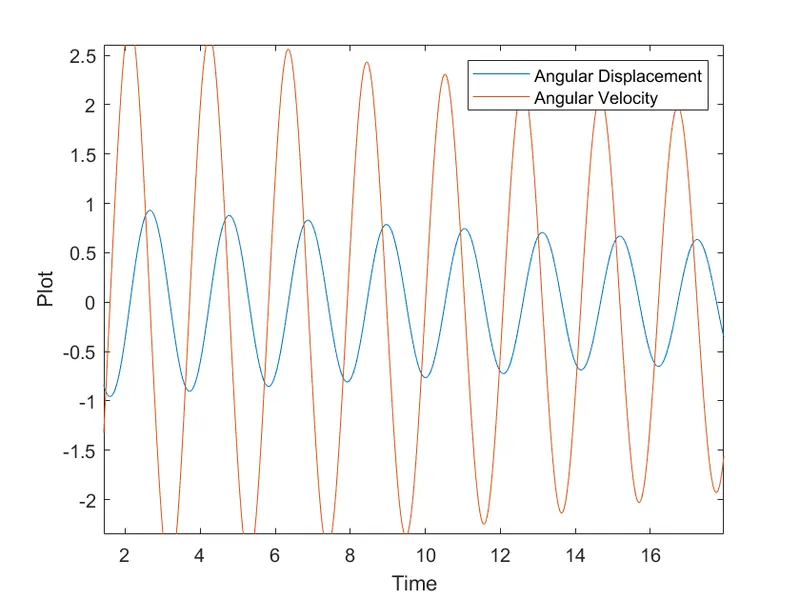
3. Plot the results obtained in the array and create the plot for Angular Displacement and Angular Velocity

4. Creathe the plot to simulate the pendulum movement back and forth

5. Create a movie and write the viedofile to create a movie clip of the pendulum movement simulation

Results:

Video Link for YouTube

Pendulum Simulation using MATLAB