Genetic Algorithm Using MATLAB

Aim: To write a program in MATLAB

Objective:

1) To write a code in MATLAB to optimise the stalagmite function and find the global maxima of the function.

2) To explain the concept of GA and explain the syntax of GA in MATLAB

3) Plot Graphs from all 3 studies for F maximum vs no of iterations

Theory:

Genetic Algortihm:

A Genetic Algorith (GA) is a method for solving both constrained and unconstrained optimization problems based on a natural selection process that mimics biological evolution. The algorithm repeatedly modifies a population of individual solutions. At each step, the GA randomly selects individuals from current population and uses them as parents to produce the children for the next generation. Over successive generations, the population "evolves" towards an optimal solution.

The GA uses 3 main types of rules at each step to create the next generation from each population

1) Selection - selects the individuals(parents) that contribute to the population at the nexe generation

2) Crossover - combines 2 parents to form children for the next generation

3) Mutation - applies randoom changes to individual parents to form children

GA Syntax:

1. x = ga(@func,nvars), where 'func" is the function name and 'nvars' is the no of variables

2. x = ga(2func,nvars,A,B,Aeq,Beq) - a set of lower and upper bounds are given so that the solution lies within that range

3. x = ga(2func,nvars,A,B,Aeq,Beq,lb,ub,nonlcon,lntCon,options), where

A,B = linear inequality contraints

Aeq,Beq = linear equality constraints

lb = lower bound

ub = upper bound

nonlcon = non linear constraints

lntcon = vector of positive integers

options = optimization options

Code:

Function:

function [f] = stalagmite(input_vector)
           x = input_vector(1);
           y = input_vector(2);
           
           f1_x = (sin(5.1*pi*x+0.5)).^6;
           f1_y = (sin(5.1*pi*x+0.5)).^6;
           f2_x = exp(-4*log(2)*((x-0.0667).^2)/0.64);
           f2_y = exp(-4*log(2)*((y-0.0667).^2)/0.64);
           
           [f] = -f1_x.*f1_y.*f2_x.*f2_y;
end

clear all
close all
clc

%Creating x and y array
x = linspace(0,0.6,150);
y = linspace(0,0.6,150);
num_cases = 50

%Creating a 2D mesh
[xx yy] = meshgrid(x,y);

%Calculating the stalagmite function
for i = 1:length(xx)
    for j = 1:length(yy)
        input_vector(1) = xx(i,j);
        input_vector(2) = yy(i,j);
        f(i,j) = stalagmite(input_vector);
        
    end
end

surfc(xx,yy,f);
xlabel('X Axis')
ylabel('Y Axis')
shading interp

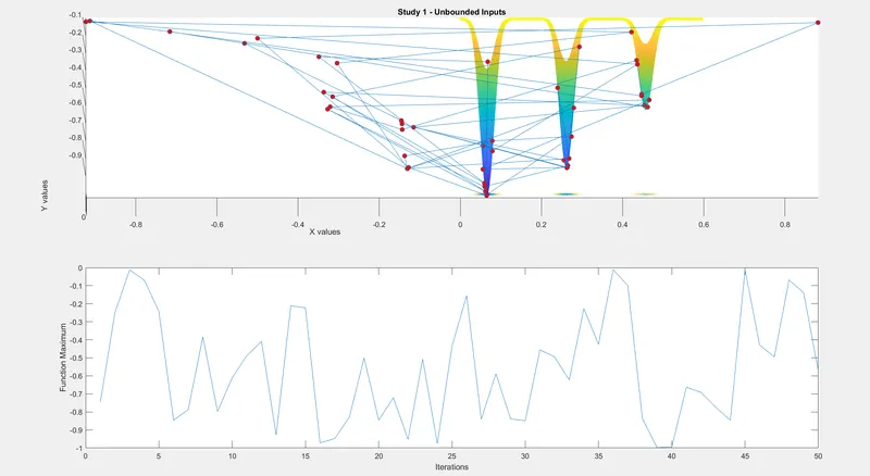
%Study 1 - Unbounded Inputs
tic
for i=1:num_cases
    [inputs,fopt(i)]=ga(@stalagmite,2);
    xopt(i) = inputs(1);
    yopt(i) = inputs(2);
end
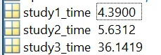
study1_time=toc
figure(1)
subplot(2,1,1)
hold on
surfc(xx,yy,f)
shading interp
title('Study 1 - Unbounded Inputs')
xlabel('X values')
ylabel('Y values')
plot3(xopt,yopt,fopt,'marker','o','markersize',6,'markerfacecolor','r')
subplot(2,1,2)
plot(fopt)
xlabel('Iterations')
ylabel('Function Maximum')

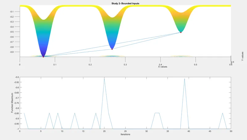
%Study 2 - with upper and lower bounds
tic
for i=1:num_cases
    [inputs,fopt(i)] = ga(@stalagmite,2,[],[],[],[],[0;0],[1;1]);
    xopt(i)=inputs(1);
    yopt(i)=inputs(2);
end
study2_time=toc
figure(2)
subplot(2,1,1)
hold on
surfc(xx,yy,f)
shading interp
title('Study 2- Bounded Inputs')
xlabel('X values')
ylabel('Y values')
plot3(xopt,yopt,fopt,'marker','o','markersize',6,'markerfacecolor','r')
subplot(2,1,2)
plot(fopt)
xlabel('Iterations')
ylabel('Function Maximum')

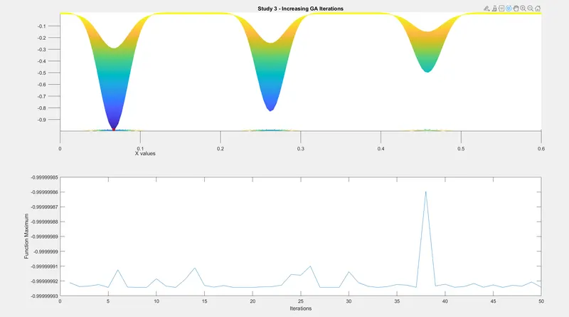
%Study 3  - Incread GA Iterations
options = optimoptions('ga')
options = optimoptions(options,'PopulationSize',500)
tic
for i=1:num_cases
    [inputs,fopt(i)] = ga(@stalagmite,2,[],[],[],[],[0;0],[1;1],[],[],options);
    xopt(i)=inputs(1);
    yopt(i)=inputs(2);
end
study3_time=toc
figure(3)
subplot(2,1,1)
hold on
surfc(xx,yy,f)
shading interp
title('Study 3 - Increasing GA Iterations')
xlabel('X values')
ylabel('Y values')
plot3(xopt,yopt,fopt,'marker','o','markersize',6,'markerfacecolor','r')
subplot(2,1,2)
plot(fopt)
xlabel('Iterations')
ylabel('Function Maximum')
       

Code Explanation:

• Create a function called stalagmite using the predefined equations
• Create an array of input variables and generate a 2D mesh using meshgrid function
• Generate the Minimas and Maximas using the stalagmite function and plot the graph
• Using the tic-toc functions, generate 3 different studies: Unbounded,Bounded and Increased Iterations
• Plot the graphs for each study

Results: