Curve Fitting using MATLAB

Aim: To write a program in MATLAB

Objective:

• To write a code in MATLAB to fit the linear and cubic polynomial for the Cp data and plot them accordingly
• To explain the parameters used to measure the fitness characteristics
• To write a code in MATLAB to show thw splitwise method

Theory:

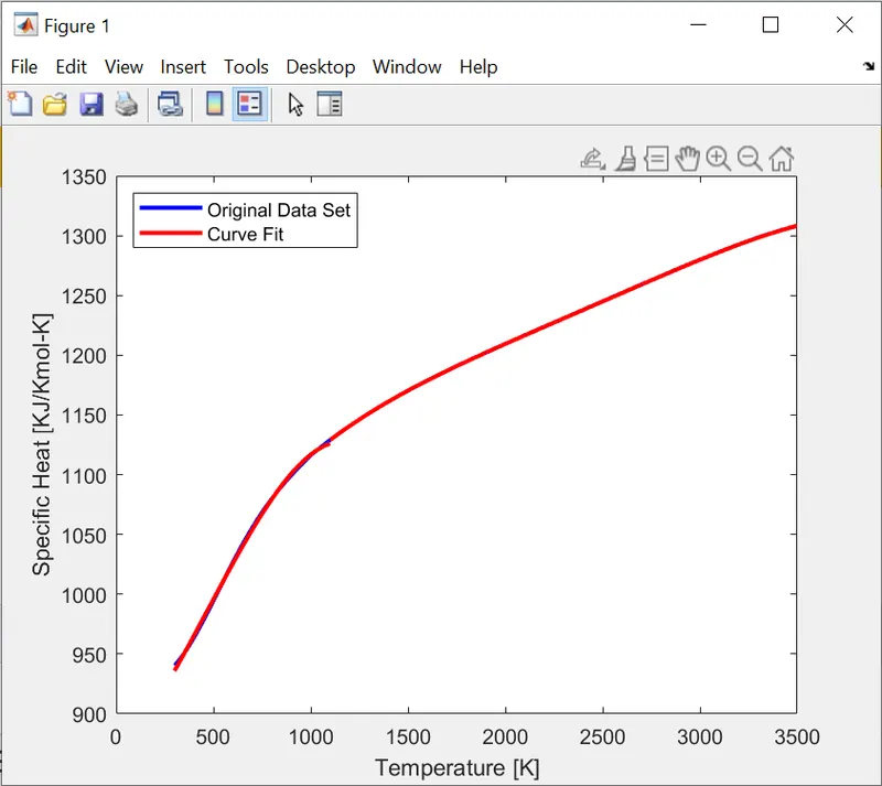
Curve fitting is the process of constructing a curve or mathematical fuicntions wich possess the closest proximity to the real series of data. By curve fitting, we can mathematically construct the functional relationship between the observed data set and parameter values.

The accuracy of the curve can be imprived by increasing the degree of the polynomial, in order to obtain a 'Best Fit'

The best fit is achieved when the geometric distances from the given points to the fitting curve are minimized. The parametric models used to measure the fitness of the curve are

1. The Sum of Squares due to Error (SSE)
2. R-Square
3. Adjusted R-Square
4. Root Mean Squared Error (RMSE)

1) Sum of Squares due to Error: Measured the total deviation of the response values from the fit to the response values.

2) R-Square:It is the square of the correlation between the response values and the predicted response values. Measures how successful the fit is in explaining the variation of the data.

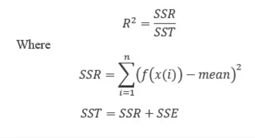
3) Adjusted R-Square: It is a normalizing variation of the R-Square, which neglects the variation due to insignificant independent variable in R-Square

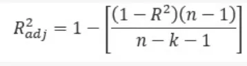
4) Root Mean Squared Error: It is an estimate of the standard deviation of the random component in data

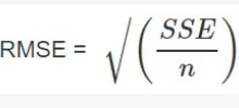
Code:

Linear Fit:

clear all
close all
clc

% Preparing the data
cp_data = load('data');
temperature = cp_data(:,1);
cp = cp_data(:,2);

% Curve fit
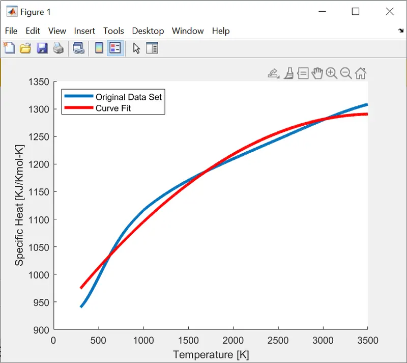
% cp = a*T^2 + b*T + c (Linear Fit)

co_effs = polyfit(temperature,cp,2);

predicted_cp = polyval(co_effs,temperature);

% Comparing curve fit with original
hold on
plot(temperature,cp,'linewidth',3)
plot(temperature,predicted_cp,'linewidth',3,'color','r')
xlabel('Temperature [K]')
ylabel('Specific Heat [KJ/Kmol-K]')
legend('Original Data Set','Curve Fit','location','northwest')

Cubic Fit:

clear all
close all
clc

% Preparing the data
cp_data = load('data');
temperature = cp_data(:,1);
cp = cp_data(:,2);

% Curve fit
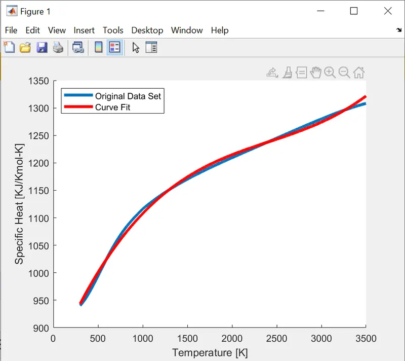
% cp = a*T^3 + b*T^2 + c*T + d (Cubic Fit)

co_effs = polyfit(temperature,cp,3);

predicted_cp = polyval(co_effs,temperature);

% Comparing curve fit with original
hold on
plot(temperature,cp,'linewidth',3)
plot(temperature,predicted_cp,'linewidth',3,'color','r')
xlabel('Temperature [K]')
ylabel('Specific Heat [KJ/Kmol-K]')
legend('Original Data Set','Curve Fit','location','northwest')

Splitwise Method:

clear all
close all
clc

% Preparing the data
cp_data = load('data');
temperature = cp_data(:,1);
cp = cp_data(:,2);


% Splitting the data
temperature1 = cp_data(1:800,1);
cp1 = cp_data(1:800,2);

temperature2 = cp_data(801:1600,1);
cp2 = cp_data(801:1600,2);

temperature3 = cp_data(1601:2400,1);
cp3 = cp_data(1601:2400,2);

temperature4 = cp_data(2401:3200,1);
cp4 = cp_data(2401:3200,2);


% Cubic fit for the given data points
co_eff1 = polyfit(temperature1,cp1,3);
pred_cp1 = polyval(co_eff1,temperature1);

co_eff2 = polyfit(temperature2,cp2,3);
pred_cp2 = polyval(co_eff2,temperature2);

co_eff3 = polyfit(temperature3,cp3,3);
pred_cp3 = polyval(co_eff3,temperature3);

co_eff4 = polyfit(temperature4,cp4,3);
pred_cp4 = polyval(co_eff4,temperature4);

% Plotting the points

plot(temperature,cp,'linewidth',2,'color','b')
hold on
plot(temperature1,pred_cp1,'linewidth',2,'color','r')
hold on
plot(temperature2,pred_cp2,'linewidth',2,'color','r')
hold on
plot(temperature3,pred_cp3,'linewidth',2,'color','r')
hold on
plot(temperature4,pred_cp4,'linewidth',2,'color','r')
xlabel('Temperature [K]')
ylabel('Specific Heat [KJ/Kmol-K]')
legend('Original Data Set','Curve Fit','location','northwest')

Code Explanation:

• Load the data from the given file and split it into temperature and cp
• Generate the co-efficient using the polyfit command and the predicted cp using the polyval command
• Plot the given data points agains teh linear and cubic polynomial results
• For the split wise method, divide the given data into 4 different data points and genereate co-efficients and predicted cp for each data point
• Plot the derived results against the original data points to get the results for best fit

Results:

Linear Fit:

Cubic Fit:

Splitwise Method: