Solving and obtaining Numerical solution to the One-dimensional Linear Convection equation using MATLAB
WEEK 4 -LINEAR CONVECTION
Objective : To solve the below mentioned 1D Linear Convection Equation using Finite Difference Method where forward differencing is used for the time derivative term and backward differencing is used for the space terms. The initial velocity and the final velocity is to be compared for various values of the number of divisions of the domain length (L), 'n' and in the end, the variation of the graphs for various 'n' values are to be discussed.
∂u∂x+C∂u∂z=0">∂u∂x+C∂u∂z=0∂u∂x+C∂u∂z=0
Now to solve it numerically, we need to implement some differencing schemes of the numerical techniques to discretize the equation.
The discretization for the first-order time derivative is given by:
∂u∂t=〖un+1〗i-〖un〗iδt">∂u∂t=〖un+1〗i−〖un〗iδt∂u∂t=〖un+1〗i-〖un〗iδt
where ∂u∂t">∂u∂t∂u∂t = First order space derivative of the velocity u,
〖un+1〗i">〖un+1〗i〖un+1〗i = Velocity profile at (n+1)th time step
〖un〗i">〖un〗i〖un〗i = Velocity profile at nth time step
The discretization of first order spacial derivative in x is given by:
∂u∂z=〖un〗i-〖un〗i-1δz">∂u∂z=〖un〗i−〖un〗i−1δz∂u∂z=〖un〗i-〖un〗i-1δz
∂u∂z">∂u∂z∂u∂z is First order space derivative of the velocity u
〖un〗i">〖un〗i〖un〗i velocity at the grid point ( i ) and time step
〖un〗i-1">〖un〗i−1〖un〗i-1 is velocity at the grid point ( i -1 ) and time step n
Now the domain Initialisations include :
L = length of the domain = 1m
c = diffusion velocity = 1m/s
Also assume, c∂t∂x=λ">c∂t∂x=λc∂t∂x=λ
This Lambda also termed as the CFL constant plays a very important in governing the stability and convergence of the numerical scheme employed.
The stability of the numerical scheme is governed by CFL Stability Criteria.
For a 1-D case, the value of the constant lambda, λ≤c">λ≤cλ≤c to ensure convergence,
where C = velocity of the propagation.
This value of the CFL constant also determines the rate of convergence and the accuracy of the numerical scheme.
The time step and the number of grid points of the domain are kept as user input in the Matlab code :
In this project, the number of the grid points is kept constant and is set to n=80. The Effect of different time step sizes is seen in the stability of the solution.
The code to solve the equation numerically in MATLAB is given below:
MATLAB CODE :
clear all
close all
clc

% Inputs fo rlnear convection problem
L = 1; %Length of the domain
n = input('Input the number of grid points that you want:'); %Nujmber of grid points
c = 1;  %Linear convection velocity
dt = input('Input the time step size(dt):'); % Time step

%Calculations part
x= linspace(0,L,n); %Mesh creation using the length of domain and number of grid points
dx = x(2)-x(1); %As the linspace creates uniform mesh diff b/w consecutives gives mesh grid
% dx= L/(n-1)
p = abs(x - 0.1);
[ min_value_start , n_start_index ] = min(p);

q = abs(x-0.3);
[ min_value_end , n_end_index ] = min(q);

%Initialising the solution arrays and applying boundary conditions
u = ones(1,n);
u(n_start_index:n_end_index ) = 2;
uold1 = u;
uold  = u;

% Inputing the time till I want the time-steps
t = input('Input the time till you want the velocity profile evaluation : ');
% number of time steps
nt = t/dt;

% first order forward differencing scheme
% creating a video file
v = VideoWriter('Linear challenge 1 with time step dt and n grid points.avi');

% changing the framerate of the video so as to have a deeper insight
v.FrameRate = 10 ;
open(v);

tic
% time loop
for k=1:nt

    % Space loop
    for i = 2:n

        % Discretization done to solve the equation
        u(i) = uold(i) - c*(dt/dx)*(uold(i) - uold(i-1));

    end

    % Updating the old velocity profile for the next time step
    uold = u;

    % plotting the velocity profile
    plot(x,u,'k','linew',2);

    % Specifying the length of the axis
    axis([0 1 -1 3]);

    % making a video file and then joining the images together
    frame = getframe(gcf);
    writeVideo(v,frame);

    % Pausing the loop to 0.02 seconds for smooth animation
    pause(0.02)

end

close(v);
  toc

 % plotting the final figures
 figure()
 plot(x,uold1,'b','linew',2);
 hold on;
 plot(x,u,'k','linew',2);
 legend('Initial Profile',[ 'Profile after 0.4 seconds for' num2str(n) ' grid points' ])
 title('Linear Convection Plots');
 xlabel('X');
 ylabel(' Velocity ');
1) For the first Input n = number of grid points = 80 and time step size dt = 1e-1
On running the MATLAB code for n = 80 grid points and time step size dt = 1e-1 the simulation is obtained as shown below:
The graph comparing the velocity profile after 0.4 seconds and the initial profile is shown below:
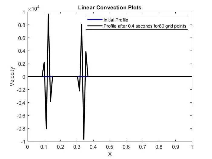
For this scheme δt=0.1 and δx=0.0127In this case the CFL constant, λ = cδtδx = 1×0.10.0127 = 7.87Clearly in this case the CFL constant is much greater than c(which is 1), and hence the numerical scheme is not stable which is seen clearly in the plots also. The solution has blown up as is seen from the values on the y-axis. It has reached an order of 10000. This type of selection of the CFL constant should be avoided as it would result in an unstable solution.
2) For the Second Input n = number of grid points = 80 and time step size dt = 1e-2
On running the MATLAB code for n = 80 grid points and time step size dt = 1e-2 the simulation is obtained as shown below
The graph comparing the velocity profile after 0.4 seconds and the initial profile is shown below:
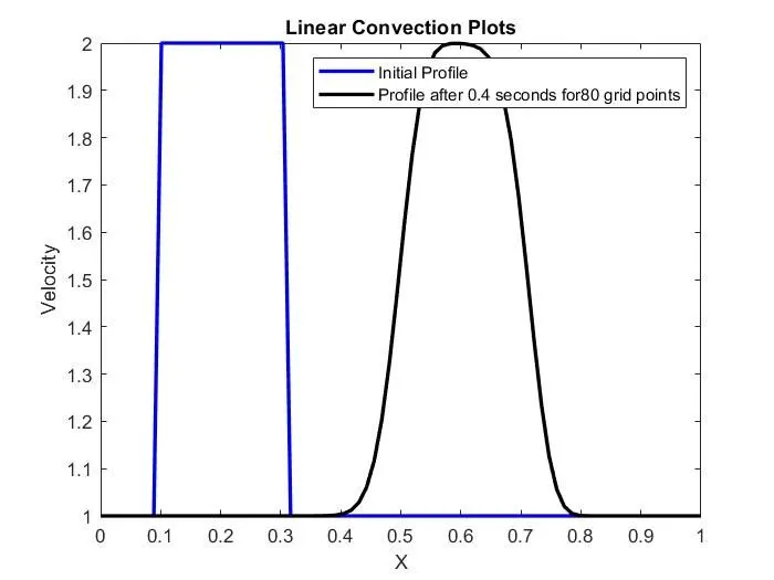
For this scheme δt=0.01 and δx=0.0127In this case the CFL constant λ = cδtδx = 1×0.010.0127 = 0.787Clearly in this case the CFL constant is less than c(which is 1), and hence the numerical scheme is stable which is seen clearly in the plots also. The solution has not blown up as is seen from the values on the y-axis. Also, it is seen that the profile after 0.4 seconds has still retained its shape to some extent as the CFL constant is more in this case.
3) For the first Input n = number of grid points = 80 and time step size dt = 1e-3 On running the
MATLAB code for n = 80 grid points and time step size dt = 1e-3 the simulation is obtained as shown below:
graph comparing the velocity profile after 0.4 seconds and the initial profile is shown below:
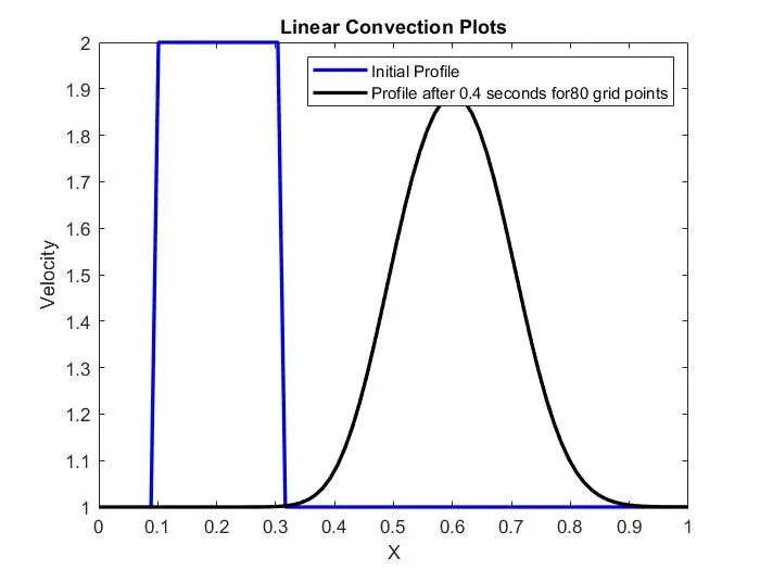
For this scheme δt=0.001 and δx=0.0127In this case the CFL constant λ = cδtδx = 1×0.0010.0127 = 0.0787Clearly in this case the CFL constant is less than c(which is 1), and hence the numerical scheme is stable which is seen clearly in the plots also. The solution has not blown up as is seen from the values on the y-axis. Also, it is seen that the profile after 0.4 seconds has lost its shape to some extent as CFL constant is less in this case as compared to the above case.
4. For the first Input n = number of grid points = 80 and time step size dt = 1e-4On running
the MATLAB code for n = 80 grid points and time step size dt = 1e-4 the simulation is obtained as shown below:
The graph comparing the velocity profile after 0.4 seconds and the initial profile is shown below:
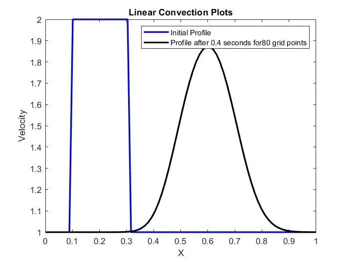
For this scheme δt=0.0001 and δx=0.0127In this case the CFL constant λ = cδtδx = 1×0.00010.0127 = 0.00787Clearly in this case the CFL constant is less than c(which is 1), and hence the numerical scheme is stable which is seen clearly in the plots also. The solution has not blown up as is seen from the values on the y-axis. Also, it is seen that the profile after 0.4 seconds has still lost its shape to quite some extent as CFL constant is less in this case as compared to the other cases.
Explanation :
1.) One interesting phenomenon to note here is the deformation of the square wave while propagating forwards. This effect can be attributed to the fact of Numerical Diffusion, a major error source in CFD studies. Numerical diffusion is the tendency for transported variables to diffuse more than they should. Theoretically, the diffusion shouldn't occur as there is no diffusion term. The square wave which was initialized in MATLAB isn't perfectly square, there is some slope in the jump of the wave. Because of this, the solution algorithm diffuses more than it should and we get a deformed profile. If we solve the problem numerically with pen and paper and account for the perfect square wave we will be able to solve with high physical consistency.
2.) Another important fact to note here is that as the time step size is decreased we see more deformation in the square wave. This is because as there are more time grid points numerical diffusion will occur in the provided time.
Conclusioin :
It is seen that the simulation time increases as the timestep decreases and it makes sense also as more computations are done in order to reach a particular value with smaller increments. The effect of the time step sizes is studied on the numerical scheme and the results are in agreement with the mathematical formulas and the conditions derived for governing them. The CFL constant also determines the rate of convergence and the accuracy of the numerical scheme. Hence the proper selection of the parameters is a must so that the CFL stability criterion is satisfied in order to solve the problem accurately and efficiently.