Sloshing in Gearbox

Aim: Simulation of fluid sloshing effect in a gear-box.

Objective:

• To understand and setup up a multiphase flow wherein fluid and structure interaction takes place.
• To understand the sloshing effect and set up the solver for the same.
• To understand the implementation of UDF utilised for defining the motion of the gears.
• To understand the concept of dynamic meshing; its importance and its use.

Introduction:

What is a gearbox?

A gearbox is a mechanical device that transmits power from an engine or motor to a driven device, such as an axle or a wheel. It uses gears to increase or decrease the speed and torque of the output shaft. Gearboxes can be found in a variety of applications, including automobiles, bicycles, industrial machinery, and power tools. They can be manual or automatic and can have multiple gears to provide different speed and torque ratios.

What is meant by lubrication and its need in a gearbox?

Lubrication is the process of applying a lubricant, such as oil or grease, to the moving parts of a gearbox to reduce friction and wear. Lubrication is essential for the proper functioning of a gearbox, as it helps to:

• Reduce friction: Lubricants form a thin film between the moving parts of a gearbox, which reduces the amount of friction between them. This helps to prevent wear and tear on the gears and bearings and makes the gearbox run more smoothly and efficiently.
• Cool the gearbox: Lubricants also help to dissipate heat from the gears and bearings, which can be generated by friction and the mechanical energy being transmitted through the gearbox.
• Protect against corrosion: Lubricants can also help to protect the gears and bearings from rust and corrosion, which can occur as a result of exposure to moisture or other environmental factors.
• Cleaning: Lubricants can also help in cleaning the gearbox by carrying away debris, dust and other contaminants that may accumulate in the gearbox.

It is important to use the correct type of lubricant for a gearbox, as different types of lubricants are designed for different types of applications and operating conditions. Also, it is important to monitor the lubricant level and to change the lubricant at regular intervals as per the manufacturer's recommended schedule. Neglecting lubrication and not using the right lubricant can lead to serious damage to the gearbox, which can be costly to repair or replace.

What is the fluid Sloshing effect? Discuss whether the sloshing effect is good or bad? Explain.

Fluid sloshing refers to the movement of fluid inside a container, such as a tank or a gearbox, when the container is subjected to external forces, such as vibrations or accelerations. The fluid inside the container can move back and forth, creating waves and impacts on the walls of the container.

The sloshing effect can have both positive and negative impacts depending on the application.

Positive impacts:

• In some applications, such as in vehicles or boats, the fluid sloshing can help to dampen vibrations and reduce the overall stress on the vehicle or boat's structure.
• Also, in some industrial processes, the fluid sloshing can be used to mix and agitate the fluid inside a tank, which can be beneficial for certain types of chemical reactions.

Negative impacts:

• In other applications, such as in tanks that store liquids, the fluid sloshing can be a problem, as it can create high loads on the walls of the tank and cause damage to the tank or its supporting structure.
• Also in gearboxes, the fluid sloshing can lead to variations in the lubricant pressure and poor lubrication of the gears, which can lead to increased wear and tear on the gears, bearings and other components.

In summary, fluid sloshing can have both beneficial and detrimental effects depending on the application. Therefore, it is important to consider the potential effects of fluid sloshing when designing tanks, gearboxes and other systems that may be subjected to vibrations or accelerations.

In this study, we examine this sloshing effect in a gearbox consisting of spur gears.

What is dynamic meshing? Give some other examples where dynamic meshing can be used.

Dynamic meshing refers to the process of adjusting the mesh, or the discretization, of a computational domain in a numerical simulation in response to the motion of the boundaries or the fluid flow. Dynamic meshing can be used in simulations of fluid flow, heat transfer, and structural mechanics, among others.

For instance, in this study, the fluid-structure interaction (of the moving gear teeth with the lubricant present in the casing), the mesh needs to adapt itself in the region where the gear teeth engage and disengage. For this purpose, dynamic meshing is used. Some other areas of application are as follows:

In fluid dynamics, dynamic meshing can be used to track the motion of interfaces, such as the free surface of a liquid or the boundary between two immiscible fluids. This allows for more accurate and efficient simulations of phenomena such as free surface flows, droplet or bubble dynamics, and multiphase flow.

In structural mechanics, dynamic meshing can be used to track the motion of bodies in contact, such as in simulations of impact, penetration, or rock fragmentation. This allows for more accurate and efficient simulations of phenomena such as penetration, fragmentation and contact mechanics.

In other fields such as biomechanics, dynamic meshing can be used to track the motion of biological structures, such as in simulations of cell dynamics, soft tissue mechanics, and blood flow in the cardiovascular system.

In general, dynamic meshing can be used in any simulation that requires tracking the motion of boundaries or interfaces, such as in simulations of fluid-structure interaction, multi-body dynamics, and contact mechanics.

What is the use of UDF?

UDF stands for User-Defined Function. In the context of computational fluid dynamics (CFD) and other numerical simulations, a UDF is a program or a subroutine that is written by the user to specify additional or custom physics or boundary conditions that are not included in the standard solver.

UDFs are often used to extend the capabilities of a CFD solver by allowing the user to define custom mathematical functions, such as source terms, that are not built into the solver. These custom functions can be used to model complex physical phenomena or to add additional functionality to the simulation.

Some examples of the use of UDFs in CFD simulations are:

• Injection of a chemical species in a reacting flow simulation
• Specifying a non-uniform heat flux on a wall
• Defining a user-specific turbulent model
• Defining a custom boundary condition
• Defining a custom initial condition

UDFs can be written in a variety of programming languages, such as C, C++, or Fortran, and are typically integrated into the CFD solver using an interface such as a library or an application programming interface (API). UDFs are a powerful tool that can be used to customize and extend the capabilities of a CFD solver, and they are widely used in the industry and research to simulate complex systems and phenomena.

In this case, the UDF was provided to define the motion of the spur gears (in terms of the angular velocity and direction).

Discuss the common errors that occurred in the simulation.

A] 'Dynamic mesh failed' error.
"Dynamic mesh failed" is an error message that can occur when running a numerical simulation that uses dynamic meshing, such as a CFD simulation that tracks the motion of interfaces or boundaries. This error message indicates that the solver was unable to update the mesh or the discretization of the computational domain according to the motion of the boundaries or interfaces.

There are several possible causes for this error, including:

• Insufficient memory or computational resources: The solver may require more memory or computational power to update the mesh, especially if the motion of the boundaries or interfaces is complex or high-frequency.
• Numerical instability: The solver may become unstable when trying to update the mesh, leading to a divergence in the solution. This can be caused by poor initial conditions, poor mesh quality, or improper boundary conditions.
• Error in the UDF: If the simulation uses a UDF to track the motion of the boundaries or interfaces, this error may indicate that there is an error in the UDF, such as a syntax error or a logical error.

To troubleshoot this error, it is important to check the solver's log or output files for more detailed information about the error and its cause. It may also be necessary to check the mesh quality, adjust the time step, review the boundary conditions, and check the UDFs for any errors. In some cases, it may be necessary to simplify the problem, reduce the complexity of the mesh, or use a different meshing algorithm to avoid the dynamic mesh failed error.

B] 'Negative cell volume detected' error.
"Negative cell volume detected" is an error message that can occur when running a numerical simulation that uses a finite volume method, such as a CFD simulation. This error message indicates that the solver has detected a cell, or a small volume of the computational domain, with a negative volume. This is a numerical issue and it can be caused by several reasons:

• Improper mesh: A negative cell volume can occur if the mesh is not properly aligned with the geometry of the problem or if the mesh is too coarse. This can be caused by poor-quality elements or irregular meshes.
• Misaligned boundary conditions: When the boundary conditions are not properly aligned with the mesh, it can cause negative cell volume.
• Non-physical solution: Negative cell volume can occur if the solution is not physically meaningful or if the simulation is diverging. This can be caused by poor initial conditions, poor boundary conditions or poor choice of numerical methods.
• Error in the UDF: If the simulation uses a UDF to specify the boundary conditions or source terms, this error may indicate that there is an error in the UDF, such as a syntax error or a logical error.

To troubleshoot this error, it is important to check the solver's log or output files for more detailed information about the error and its cause. It may also be necessary to check the mesh quality, adjust the time step, review the boundary conditions, and check the UDFs for any errors. Also, it may be necessary to use a more refined mesh or re-run the simulation with different numerical settings.

Workflow:

1. Preparing the geometry
2. Generate mesh for the geometry
3. Setting up the solver
4. Setting up the solution monitors
5. Post-processing to observe the results

Ansys Fluent:

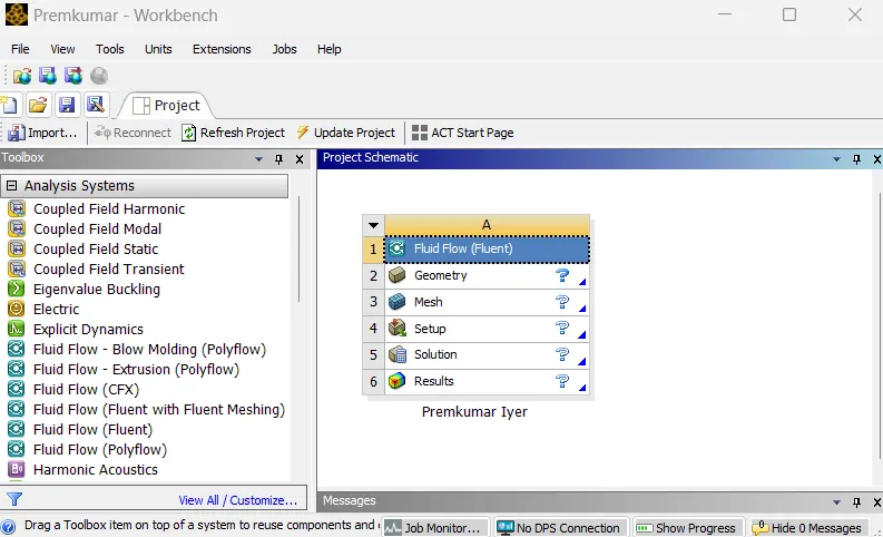In the Ansys workbench project window, Fluid Flow (Fluent) is dropped into the workspace.

Preparing the geometry:

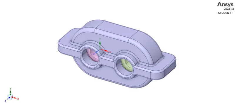
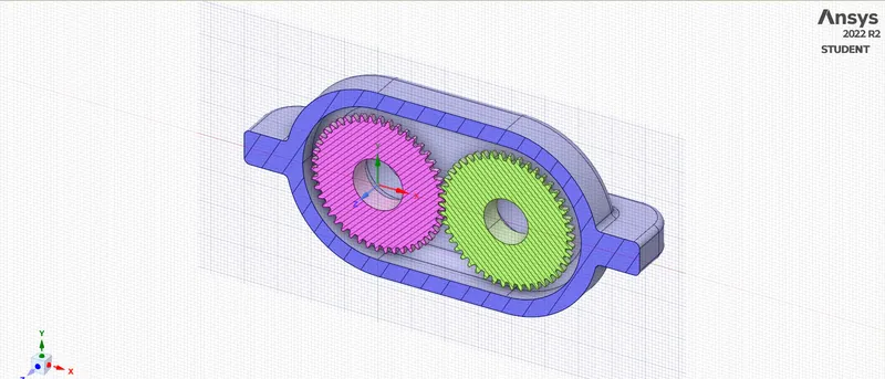
The geometry provided		Cross-sectional view

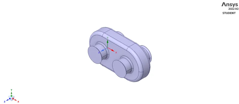
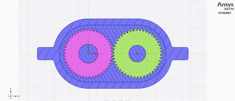
The geometry, as shown (provided as a STEP file) is imported in SpaceClaim. The CAD preparation begins with defining the fluid volume. For this, we carefully select the edges to define the internal volume, wherein these solid parts of the gearbox are not present. The volume extract tool under the prepare tab helps to do so. Thus, we obtain the following:

Volume Extract		Cross-section view

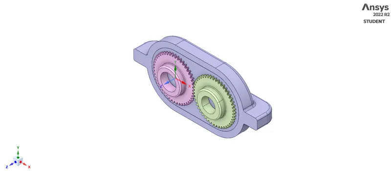
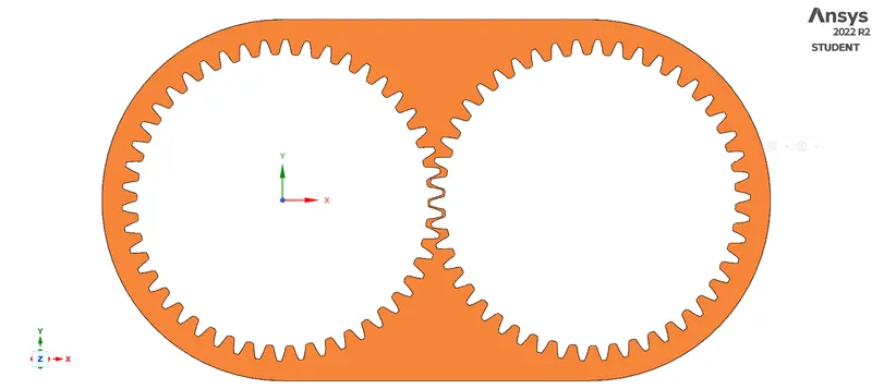
Working with a 3D model would be time consuming and highly resource exhaustive, and hence, this 3D domain is converted to 2D domain. If we carefully look at the above cross-sectional view, the region between the gears and the housing is of our importance, and hence, we need this region to be our computational domain. To do this, we use the split body command from the design tab, and once the body is reduced to half, we copy this face (coloured in amber in the figure below) and paste it into another Spaceclaim window to obtain the computational domain.

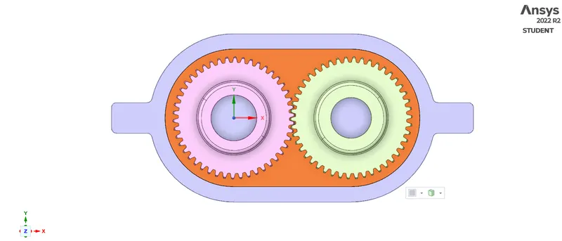After the body has been splitted	The region of interest
The computational domain

Generating mesh:

Meshing is the process, wherein the geometry is divided into smaller parts which are known as elements so that the iterative solver can solve the governing equations across the domain. In the meshing utility, a baseline mesh of the default element size is created with capture curvature turned ON. In order to improvise the mesh (since baseline mesh is a mixture of triangles and squares), the mesh method is inserted as "all triangles" and the element size is changed to 30mm. This gives 15994 number of elements and the generated mesh and its metrics are as shown below:

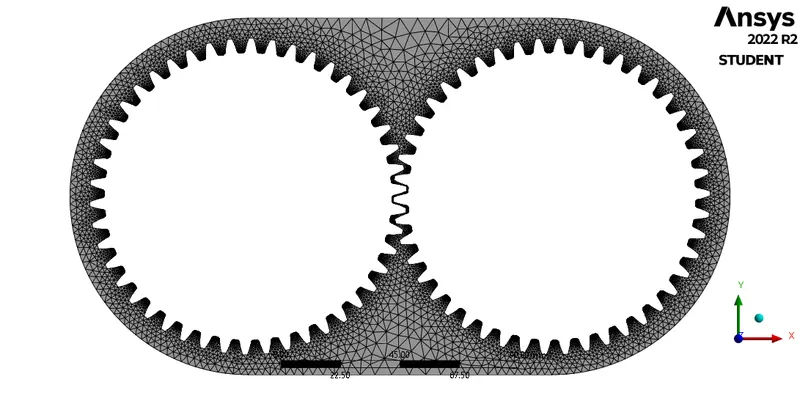The generated mesh
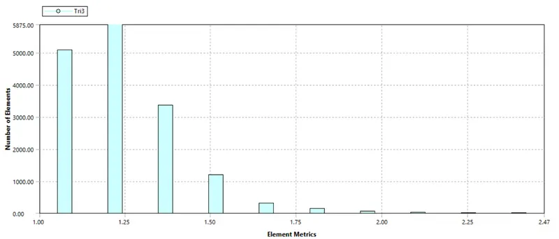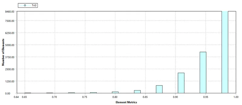Aspect Ratio	Orthogonal Quality

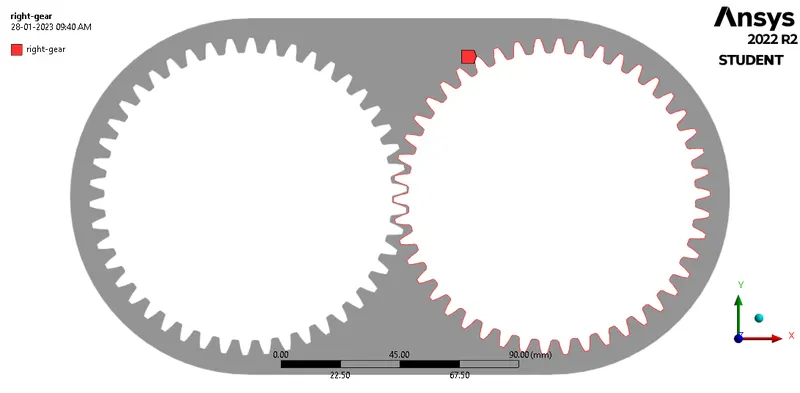
For implementing the boundary conditions, the "boundaries" must be clearly defined. To do so, the mesh utility itself has a tool; named selections. By selecting the respective edges, the left gear and the right gear were defined.

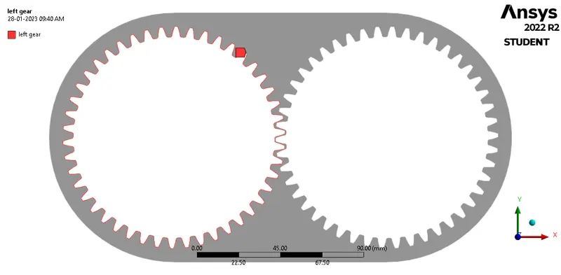Setting up the solver:

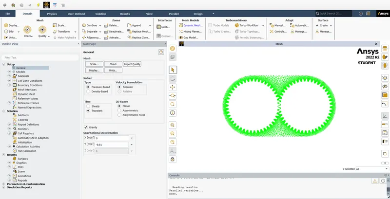An important part of a CFD simulation, the setup for the solver is done to obtain the solution. Firstly, the units of important parameters are set to desired units (preferably SI units). In the general setup, a transient-state (since, we have to enable dynamic mesh) pressure-based solver is utilised and gravity is enabled in the y-direction (-9.81`m//s^2)`. The required materials re imported from the Fluent database (engine oil for the first case and n-heptane for the second case.

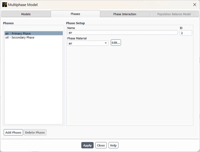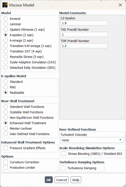
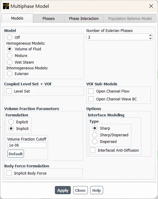
In the models tab, in the viscous models, the `k-epsilon` realizable with enhanced wall treatment is enabled. In the same tab, the multiphase option is clicked on. In this, the volume of fluid method with two Eulerian phases is selected. Further, the formulation is switched to implicit to overcome the Courant number restrictions on the time step. The air is defined as the primary phase and oil as the secondary phase. Once this is done, the multiphase window is closed.

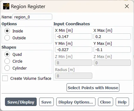The region where the fluid would be present has to patched and for this we need to define the region filled with fluid. To do this, cell register is created (an option in the solution tab). The register is made based on the inside volume and the shape of register is quad. And the following result is obtained:

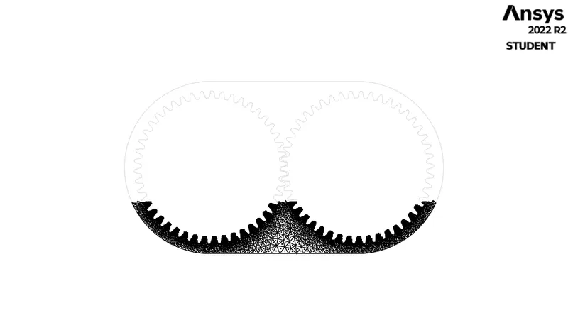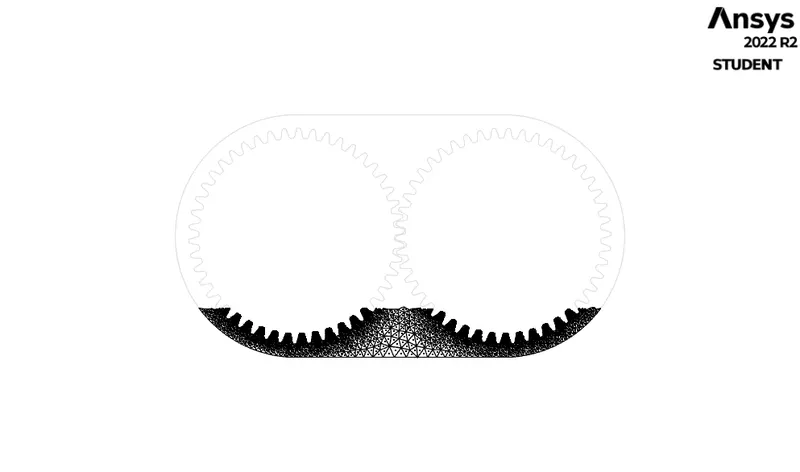For 30% immersion	For 20% immersion

#include "udf.h"

DEFINE_CG_MOTION(right_motion, dt, vel, omega, time, dtime)
{
	vel[0] = 0.0;
	vel[1] = 0.0;
	vel[2] = 0.0;

	omega[0] = 0.0;
	omega[1] = 0.0;
	omega[2] = 2.0e2; /* [rad/s]*/
}
DEFINE_CG_MOTION(left_motion, dt, vel, omega, time, dtime)
{
	vel[0] = 0.0;
	vel[1] = 0.0;
	vel[2] = 0.0;

	omega[0] = 0.0;
	omega[1] = 0.0;
	omega[2] = -2.0e2; /* [rad/s]*/
}

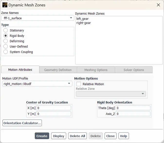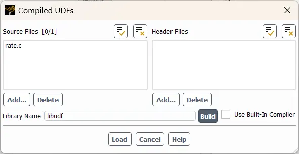
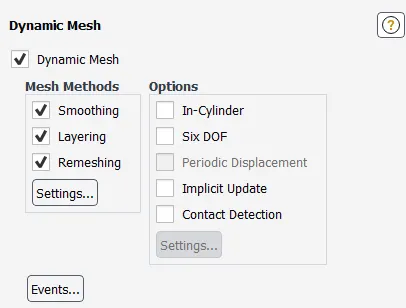
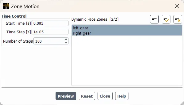
The above code snippet is used in the UDF file that defines the motion of the gear. The file is imported from the options under the user-defined tab, and after adding the file, click on build and then load the file in the solver workspace. Then under the setup tab, the dynamic mesh is enabled and the dynamic mesh zones are created based on the zone name, the motion type as a rigid body and the centre of gravity of the gear. Later, we ensure the motion is properly set by previewing the motion of the gears.

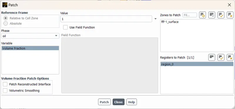
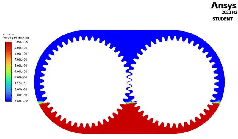
And, thus the solution is initiated by standard initialisation and the regions in the computational domain are patched to define the fluid region. The domain is patched with a volume fraction (for oil) of zero and in the register as 1. Contour is displayed to ensure that the regions are patched correctly.

/solve/set/time-step 0.00001
/solve/dual-time-ite 300 20 2 
/solve/set/time-step 0.00002
/solve/dual-time-ite 300 20 2 ok
/solve/set/time-step 0.00003
/solve/dual-time-ite 300 20 2 ok
/solve/set/time-step 0.00004
/solve/dual-time-ite 300 20 2 ok
/solve/set/time-step 0.00005
/solve/dual-time-ite 300 20 2 ok
/solve/set/time-step 0.00006
/solve/dual-time-ite 300 20 2 ok

The above is the journal file that is imported into the solver. This is done because the larger time step values will cause float point errors and a lower value would take considerably longer time to compute the results. This enables us to smoothly increase the time step value so that the same flow time is achieved in a lesser time and number of steps.

Post-processing (Results):

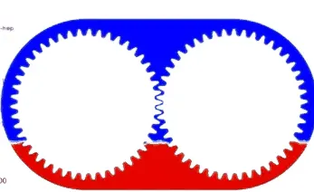
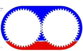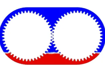n-heptane (20% immersion)	engine oil (20% immersion)
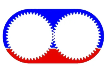n-heptane (30% immersion)	engine oil (30% immersion)

Conclusion(s):

• The density of the fluid in a gearbox can have a significant impact on the behaviour of fluid sloshing in a gearbox simulation. The fluid density also affects the magnitude of the forces acting on the gears, which can impact the gear dynamics and the gearbox performance.
• When the fluid density is high, the sloshing motion is expected to be less severe as the fluid will have more inertia, which will make it more difficult to move. As a result, the amplitude of the sloshing motion will be smaller and the frequency will be lower. On the other hand, when the fluid density is low, the sloshing motion is expected to be more severe, with higher amplitude and frequency.
• It is important to note that the fluid-structure interaction and the gear dynamics need to be accurately modelled to obtain a reliable simulation. The use of dynamic meshing can also be useful in simulating fluid sloshing in a gearbox, as it allows the mesh to adapt to the motion of the gears and the fluid. However, care must be taken to ensure that the mesh remains of high quality and that the dynamic meshing algorithm does not introduce numerical errors.
• Overall, simulating fluid sloshing in a gearbox can be a complex task that requires careful consideration of the physics, the numerical methods, and the boundary conditions. However, with the appropriate tools and techniques, it is possible to obtain accurate and reliable predictions of the behaviour of the gearbox, which can help to optimize the design and improve the performance of the gearbox.

References:

• Introduction to GUI based CFD using Ansys Fluent - Course provided by Skill-Lync
• Ansys Inc.
• Supporting Material: Slosh Dynamics
• Supporting Material: Dynamic Mesh Update Methods
• Supporting Material: A-TO-Z GUIDE TO THERMODYNAMICS, HEAT & MASS TRANSFER, AND FLUIDS ENGINEERING
• Supporting Material: LearnCAx
• Supporting Material: Fluid Mechanics - Frank M White
• Supporting Material: Fluid Mechanics: Fundamentals and Applications - Y Cengel and J Cimbala
• Supporting Material: Fundamentals of Multiphase Flows - Christopher E. Brenner