Simulink Equation Modeling and Suspension Comparison

AIM:

To plot a function using basic Simulink blocks and to run and study a Simulink example ‘Suspension System Comparison’.

The function to be plotted is given as:

``y(x)=(x-1)*(x-3)^2*(x-9)^2`

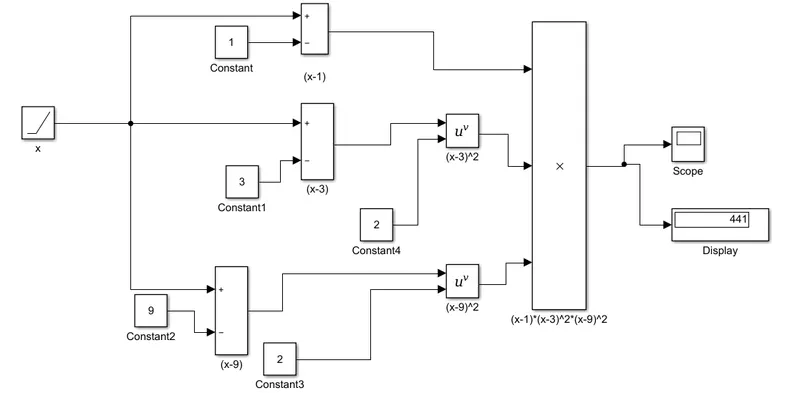
Blocks used:

Constant block:Generates a constant value

Ramp block:Generate constantly increasing or decreasing signa

Scope block:Display plots from signals generated during simulation

Add block: Adds or subtracts inputs

Display block:Shows value for its input

product block:Multiply and divide scalars and nonscalar

Steps:

1. The function is splitted into three parts: first part is `(x-1)` , second part is`(x-3)^2` , third part is `(x-9)^2`. Then the three parts can be multiplied to get the final answer of the function
2. First we Drag a ramp function from the library browser as it continously increases with time so it can act as a variable .By default value of slope is 1, so the ramp block will increase by 1 for every second of the simulation run time. Initial value and intial time for starting the ramp block is set to 0 by default.
3. Then we drag the constant block and edit it so it generates the constants 1,3,9
4. In order to be able to square the second and third term of the equation, the output of the sum block of the second and third term is linked to a Math function block and by double clicking it we have selected squaring math function in that block.
5. So output now represents (x-1), (x-3)^2, (x-9)^2 respectively. As per the equation we have multiply all these terms to get the final value of the given function.
6. So these outputs are given as inputs to a product block. This block multiplies all the inputs and gives product of these inputs as output. Thus the output of product block will be (x-1)*(x-3)^2*(x-9)^2.
7. Now to display the output of this product block, we have connected output of this block to Display block, which will display the result. For getting a graph, same output of the is connected to the scope block, which will generate a graph representing the value of the function for each second of time.
8. Then we adjust the simulation time at 10 s and press run to run the simulation

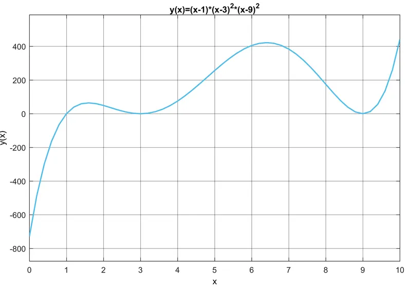
Model verification:

The Display in the last step showed the value of 441,this can be used to verify the model by simply substituting X with 10 in the main equation:`(10-1)*(10-3)^2*(10-9)^2=9*49=441`

Suspension System Comparison:

AIM:

• To know the objective of the simulation and the similarity and differences betwee the models
• To observe the results
• To explain how the velocity source was generated

Introduction:

Sprung mass: It is the portion of the vehicle's total mass that is supported above the suspension, including in most applications approximately half of the weight of the suspension itself. The sprung mass typically includes the body, frame, the internal components, passengers, and cargo, but does not include the mass of the components at the other end of the suspension components.

Unsprung mass: It is the mass of the suspension, wheels or tracks (as applicable), and other components directly connected to them, rather than supported by the suspension. It includes the mass of components such as the wheel axles, wheel bearings, wheel hubs, tires, and a portion of the weight of driveshafts, springs, shock absorbers, and suspension links. If the vehicle's brakes are mounted outboard (i.e., within the wheel), their mass is also considered part of the unsprung mass.

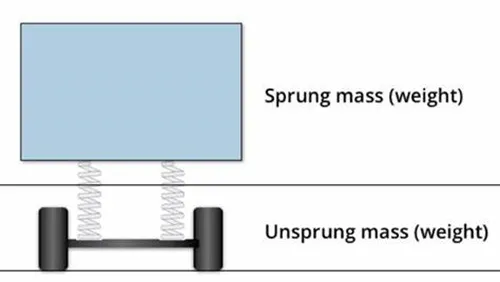
suspension components:

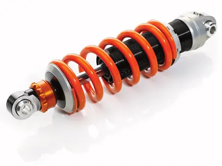
Shock absorber:

It is a mechanical or hydraulic device designed to absorb and damp shock impulses. It does this by converting the kinetic energy of the shock into another form of energy (typically heat) which is then dissipated. Most shock absorbers are a form of dashpot (a damper which resists motion via viscous friction

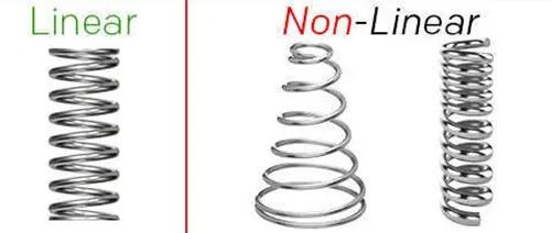
Non-linear spring:

Non-linear springs are helical coil springs that exert an inconsistent amount of force (equation is not f=kx) as it is under a working load or torque. This means that the force needed to travel one inch, millimeter, or degree might not double when it travels two inches, millimeters, or degrees like a linear spring would.This is done by variable diameter coils and variable thickness wires

variable spring:

The spring that can be adjusted via a screw to generate variable initial force or preload

Model objective:

The Objective the simulation is to observe how the three set of springs will respond to the oscillating velocity source and to determine which one will be suited for the input frequencies provided by the input.

Model similarities and differences:

Similarities: All models have the same input and all have the same tyre model represented as a linear translational spring (F=kx)and has the same sprung and unsprung masses

Differences:One model depends only on the shock absorber to deal with road irregularities,while the other depend on non-linear spring and damper which their force equation depend on polynomial function and the last one depend on variable spring which is adjusted to ensure critical damping is met

Blocks used:

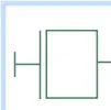Mass block:This block represents an ideal translational mass

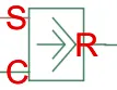Force source block:This block represents an ideal source of force that generates force propotional to input physical signal

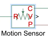Motion sensor block:represents and ideal translational motion sensor

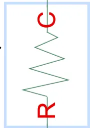
Shock absorber block: Represents a translational shock absorber

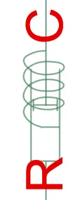
Non linear trasnlational spring block:This block models a non linear translational spring with polynomial force equation

Non linear translational damper block:Models a non linear damper with ploynomial force equation

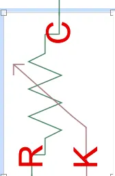Variable tanslational spring block:Models a linear variable translational spring

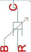
Variable translational damper block:Models a linear variable translational damper

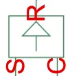Velocity source block:Ideal translation velocity source

Goto block:send signals from blocks that have the specified tag (normal simulink signal)

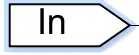From block : Receives signal from the goto block with the specified tag (normal simulink signal)

pmc_port (connection port)block:for routing physical signal

ps simulink converter block: Convert physical signal into Simulink input signal

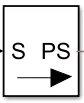Smulink ps converter block: convert simulink signal into physical signal

Inport block:provide input for subsystem or model

Outport block:provide output for subsystem or a model

Mux block:Combine input signals of same data type and complexity into virtual vector

Demux block:Extract and output elements of virtual vector signal

Rate transition block :handle transfer of date between ports operating at different rates

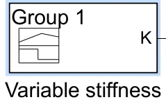signal builder:create and generate interchangebale groups of signals whose waveform are piecewise linear

Mechanical translation reference block:It represents a mechanical translation reference point

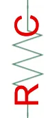Translational spring block: The block represents an ideal mechanical linear spring

Input parameters:

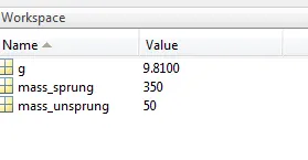
The gravity ,sprung and unsprung mass are the input values which were created from the masking process,it should also be noted that the value in the masking is defined as mass_sprung and mass_unsprung,so they are used directly to write any equation or input instead of numerical values

Block Masking:

A mask is a custom user interface for a block. By masking a block the block diagram is encapsulated to have its own parameter dialog box with its own block description and can be changed from matlab work space

Masked mass block :

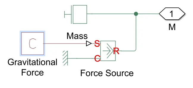
The sprung and unsrung mass blocks are masked blocks that contain the inertial mass and force of gravity generator which is connected the ps constant block that generates the weight and this is inputed in the s physical signal input and it is compared to the mechanical translation signal at the conserving port c and then output at conserving port r and they are routed via pmc_block

Motion sensor subblock:

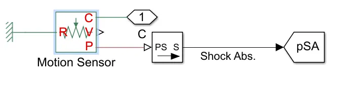
The motion sensor takes routed signal from mass block as moving rod case (c)and then it is compared to its mechanical reference (R )and then its output physical signal is converted to normal signal via ps simulink converter and then it is send via the goto block

control system sub block:

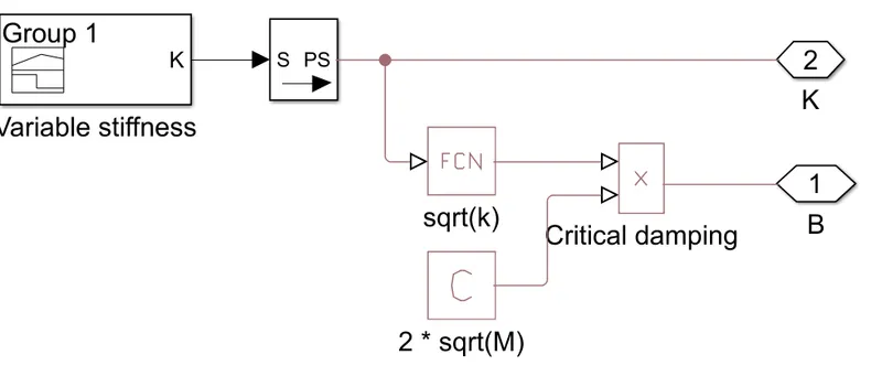
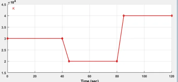Figure:variable stiffness input plot

Generates a variable stiffness value via signal builder that is changing with time ,this value is then transfered into physical signal by simulink ps converter then it is sent to the variable spring via pmc_port and it is also used to calculate the critical damping which is sent to the variable damper via also the pmc_port

Signal analyzer sub block:

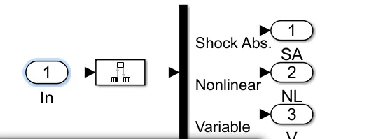
It takes the muxed shock absorber,nonlinear,and variable signal via inport input block and then it inputs it into the rate tansition block in order to be able to handle data transition at different rates and then it goes to the demux blocks which separates it into the shock absorber ,and non linear and variable spring value which are outputted from the subblock via the outport block

Velocity input sub block:

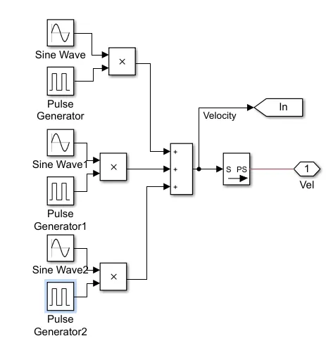
The velocity signal is generated via a combination of sine waves and pulse generators using this equation: sinewave*pulse genrator+sinewave1*pulse generator1+sinewave 2*pulse generator2

Then the simulink signal is sent to the input of the scope via goto block and the it is converted into physical signal via simulink ps converter and send via pmc_port

specification of the signals that were used to generate the input:

	Equation	Amplitude	Frequency
Sine Wave	0.1 sin(3t)	0.1	5
Sine Wave1	0.1 sin(15t)	0.1	15
Sine Wave2	0.1 sin(75t)	0.1	75

sine wave signals values

	Amplitude	Period (sec)	Pulse Width (% of period)	Phase Delay (sec)
Pulse Generator	1	120	100/6	0
Pulse Generator1	1	120	100/6	120*2/6
Pulse Generator2	1	120	100/6	120*4/6

pulse generator signal values

Model overall function:

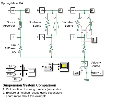
• The velocity input is introduced in the model
• Then it gets to all the three models via the tyre translational spring model which models the unsprung mass which have initial value of 50 kg
• Then it get to the spring and damper elements,and In the variable spring and damper model,an open loop control system is implement which adjusts the system to the critical damping
• Then the position of the mass which has initial value of 350 kg is sent from the translational motion sensor via goto block and it is used in the scope as an input via the from block

Model output:

Observation:

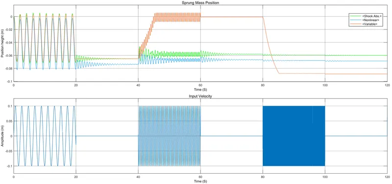
From t=0 to t=20:All models express high oscillations with non linear spring damper showing the highest amplitude

From t=20 to t=40:the variable spring damper oscillations die rapidly while the shock absorber and non linear spring damper continue

From t-40:t=60:the non linear spring damper and shock absorber models shows close response while the variable spring damper suddenly returns to zero position ,this sudden large shift may have negative consequence on passenger comfort and vehicle dynamics

From t=60 to t=80:The variable spring oscillations die rapidly while the shock absorber and non linear spring continue

From t=80 to t=100:Again the variable spring damper makes a drastic response in the opposite direction while the shock absorber and nonlinear spring damper has close response

From t=100 to t=120:Again the small vibrations of the variable spring damper die rapidly while it takes longer for the shock absorber and for the non linear spring damper to damp the oscillations.

Power Spectral Density (PSD) :

It is the measure of signal's power content versus frequency. A PSD is typically used to characterize broadband random signals.it shows the strength of the variations(energy) as a function of frequency. In other words, it shows at which frequencies variations are strong and at which frequencies variations are weak,and its unit is dpm/Hz which is a unit of level used to indicate that a power level is expressed in decibels (dB) with reference to one milliwatt (mW)

Output curve

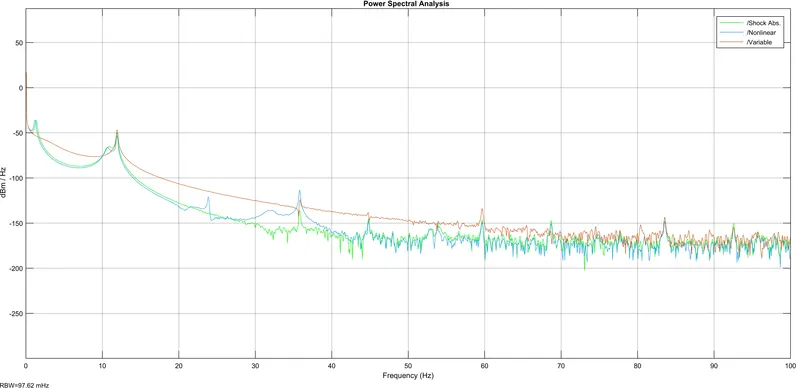
Overall:the variable spring damper shows highest power spectral density and this is confirmed by the position graph which showed huge and sudden variation of its amplitude followed by the non linear spring damper,and then the shock absorber despite being the simplest of the three types . Also the curve shows an overall trend where the PSD decrease with increasing frequency.

Studying harmonics at input frequencies:

Psd curve peaks can indicate resonance so we should look at the frequencies which the suspension models was subjected to in order to know if it is safe or not to operate in this region.

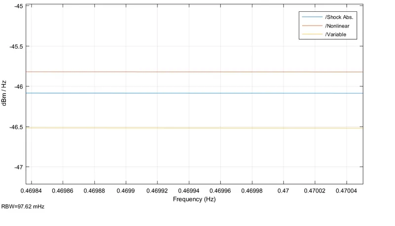
At T=0 to T=20: the frequency of the input is approximately 0.47 HZ, so it lies in the far left of the Psd curve next to the first peak in the curve which indicates it is a near resonance region in which the passenger can experience great discomfort and the overall vehicle dynamics and road contact ability will suffer,in this region in the position plot the non linear spring damper has the largest amplitude and this is now confirmed in the psd plot as it has the highest power spectral density of -45.8 dbm/Hz,followed by the shock absorber and then the variable spring damper at -46.2 and -46.6 respectively,this is the only region that it is advisable to use the variable spring damper despite it has a small advantage.

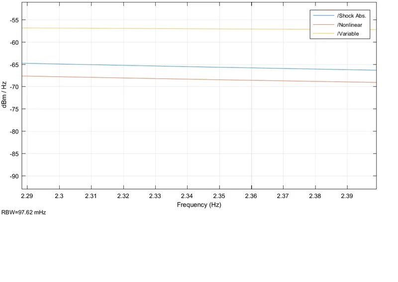
At t=40 to t=60: The frequency is approximately 2.36 Hz ,in this region the highest psd is the variable spring at -56 dbm/hz then the shock absorber and non linear spring at-65dpm/hz and -68dbm/hz respectively,This the safest and most comfortable region for the passenger for all the suspension models

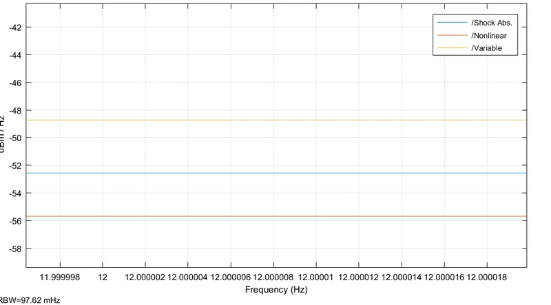
At t=80 to t=100:The frequency in this region is 12 Hz which located at the second peak which indicates resonance region which again can be uncomfortable for passenger and unsafe for the vehicle, the psd of the variable spring damper reaches-48.5 dbm/hz while the shock and the nonlinear spring damper reached -52.5 and -55.8 dpm/hz respectively

Conclusion:

The shock absorber suspension despite its simplicity showed a stable performance across the frequencies of the input source,so it should be chosen as it provides good performance and should save costs,on the other hand the variable spring damper with open loop control showed the worst performance despite its complexity because of the nature of its critical damping ,as it wants to damp any oscillation and to return to the steady state as fast as possible,this can damp small oscillations but on the expense of sudden jerks which can be uncomfortable and annoying to the passengers and it can negatively affect the vehicle handling.

Matlab function model link:

https://drive.google.com/file/d/1AXIXKgED8sS5GPHvQ_e8q9LeczVTiwsp/view?usp=sharing

Reference:

Matlab help