Simulation of Flow through a pipe in OpenFoam
Aim : Simulation of Flow through a pipe in OpenFoam and validate the results using Hagen- Poiseuille's equation.
Introduction : Here we are considering a section of pipe with an angle of 3 degrees, and assuming an axi-symmetric flow across a wedge. The flow is laminar and the Renold's no is 2100. Radius of the pipe is 0.01 metres
Procedure : In order to create geometry we specify the co-ordinates in the blockMeshDict file. And here I have generated a Matlab code to produce a blockMeshDict file which can be copy pasted to the OpenFoam, directly. I have used File parsing method to create the file. Also computed the hydrodynamic length , V_max, V_average (velocities) and shear stress.
The code to compute the physical properties and create a file for blockMeshDict is as follows :
clc
close all
clear all

R_e = 2100;  % renold's no.
rho = 1000;  % (in kg/m^3)
d = 0.001;
R = d/2   % in meters
theta = 3;
b1 = R*cosd(theta/2);
b2 = R*sind(theta/2);
L = 0.05*R_e*d + 0.095;
L_e = 0.05*R_e*d;
%L = 2.4
mu =  0.000890    %8.90*10^-4 Pa-S dynamic viscocity of water
nu = mu/rho    % kinematic viscocity of water
V_avg = (R_e*mu)/(rho*d);
V_max = 2*V_avg;

delta_pressure = (8*mu*0.095*V_avg)/R^2;   % L is after fully developed
delta_p = (delta_pressure)/rho  % for openfoam

% shear stress at the hydrodynamic length
% tau = -((delta_p)/(L))*(0.02/2);

r = linspace(0,R,100);
for i = 1:100
tau(i) = 2*mu*V_max*(abs(R/(R^2)));
u(i) = 2*V_avg*(1-r(i)^2/R^2);
end


figure(1);
plot(r,tau);
xlabel('R');
ylabel('tau');

% file parsing for blockMeshdict

a1 ='  /*--------------------------------*- C++ -*----------------------------------*';
a2 ='  =========                 |';
a3 ='        /  F ield         | OpenFOAM: The Open Source CFD Toolbox';
a4 ='       /   O peration     | Website:  https://openfoam.org';
a5 ='      /    A nd           | Version:  9';
a6 ='     /     M anipulation  |';
a7 ='  *---------------------------------------------------------------------------*/';

% vertices
v0 = [0 0 0];
v1 = [0 b1 b2];
v2 = [0 b1 -b2];
v3 = [L 0 0];
v4 = [L b1 b2];
v5 = [L b1 -b2];


f1 = fopen('blockMeshDict.txt','w')
fprintf(f1, '%s n',a1);
fprintf(f1,'%s n',a2);
fprintf(f1,'%s n',a3);
fprintf(f1,'%s n',a4);
fprintf(f1,'%s n',a5);
fprintf(f1,'%s n',a6);
fprintf(f1,'%s n',a7);

fprintf(f1,'FoamFilen{n');
fprintf(f1,'%10s %10sn','format','ascii;');
fprintf(f1,'%9s  %15sn','class','dictionary;');
fprintf(f1,'%10s %18sn','object','blockMeshDict;');
fprintf(f1,'%sn','}');
fprintf(f1,'%sn n',  '// * * * * * * * * * * * * * * * * * * * * * * * * * * * * * * * * * * * * * //')
fprintf(f1,'%snn','convertToMeters 1;');

fprintf(f1,'%sn','vertices');
fprintf(f1,'%sn','(');
fprintf(f1, 't(%d %d %d)n',v0);
fprintf(f1, 't(%d %d %d)n',v1);
fprintf(f1, 't(%d %d %d)n',v2);
fprintf(f1, 't(%d %d %d)n',v3);
fprintf(f1, 't(%d %d %d)n',v4);
fprintf(f1, 't(%d %d %d)n',v5);
fprintf(f1,'%snn',');');

fprintf(f1,'%sn','blocks');
fprintf(f1,'%sn','(');
fprintf(f1,'%20s %s %sn','hex (0 3 5 2 0 3 4 1)','(100 10 1)','simpleGrading (0.75 0.25 1)');
fprintf(f1,'%snn',');');

fprintf(f1,'%sn','edges');
fprintf(f1,'%sn','(');
fprintf(f1,'%10s (0 %d 0) n','arc 1 2',R);
fprintf(f1,'%10s (%d %d 0) n','arc 4 5',L,R);

fprintf(f1,'%snn',');');

fprintf(f1,'%sn','boundary');
fprintf(f1,'%sn','(');
fprintf(f1,'%7sn','axis');
fprintf(f1,'%7sn','{');
fprintf(f1,'%17sn','type empty;');
fprintf(f1,'%15sn','faces');
fprintf(f1,'%10sn','(')
fprintf(f1,'%20sn','(0 3 3 0)');
fprintf(f1,'%10sn',');')
fprintf(f1,'%7sn','}')

fprintf(f1,'%7sn','wall');
fprintf(f1,'%7sn','{');
fprintf(f1,'%17sn','type wall;');
fprintf(f1,'%15sn','faces');
fprintf(f1,'%10sn','(');
fprintf(f1,'%20sn','(4 5 2 1)');
fprintf(f1,'%11sn',');');
fprintf(f1,'%7sn','}');

fprintf(f1,'%7sn','inlet');
fprintf(f1,'%7sn','{');
fprintf(f1,'%17sn','type patch;');
fprintf(f1,'%15sn','faces');
fprintf(f1,'%10sn','(');
fprintf(f1,'%20sn','(0 1 2 0)');
fprintf(f1,'%11sn',');');
fprintf(f1,'%7sn','}');

fprintf(f1,'%7sn','outlet');
fprintf(f1,'%7sn','{');
fprintf(f1,'%17sn','type patch;');
fprintf(f1,'%15sn','faces');
fprintf(f1,'%10sn','(');
fprintf(f1,'%20sn','(3 5 4 3)');
fprintf(f1,'%11sn',');');
fprintf(f1,'%7sn','}');

fprintf(f1,'%7sn','wedgeFront');
fprintf(f1,'%7sn','{');
fprintf(f1,'%17sn','type wedge;');
fprintf(f1,'%15sn','faces');
fprintf(f1,'%10sn','(');
fprintf(f1,'%20sn','(3 4 1 0)');
fprintf(f1,'%11sn',');');
fprintf(f1,'%7sn','}');

fprintf(f1,'%7sn','wedgeBack');
fprintf(f1,'%7sn','{');
fprintf(f1,'%17sn','type wedge;');
fprintf(f1,'%15sn','faces');
fprintf(f1,'%10sn','(');
fprintf(f1,'%20sn','(0 2 5 3)');
fprintf(f1,'%11sn',');');
fprintf(f1,'%7sn','}');

fprintf(f1,'%snn',');');

fprintf(f1,'%sn','mergePatchPairs');
fprintf(f1,'%sn','(');
fprintf(f1,'%snn',');');
fprintf(f1,'%sn','// ************************************************************************* //');
the following text will be generated once we execute the above code :
  /*--------------------------------*- C++ -*----------------------------------*
  =========                 |
        /  F ield         | OpenFOAM: The Open Source CFD Toolbox
       /   O peration     | Website:  https://openfoam.org
      /    A nd           | Version:  9
     /     M anipulation  |
  *---------------------------------------------------------------------------*/
FoamFile
{
    format     ascii;
    class      dictionary;
    object     blockMeshDict;
}
// * * * * * * * * * * * * * * * * * * * * * * * * * * * * * * * * * * * * * //

convertToMeters 1;

vertices
(
	(0 0 0)
	(0 4.998287e-04 1.308847e-05)
	(0 4.998287e-04 -1.308847e-05)
	(2.000000e-01 0 0)
	(2.000000e-01 4.998287e-04 1.308847e-05)
	(2.000000e-01 4.998287e-04 -1.308847e-05)
);

blocks
(
hex (0 3 5 2 0 3 4 1) (100 10 1) simpleGrading (0.75 0.25 1)
);

edges
(
   arc 1 2 (0 5.000000e-04 0)
   arc 4 5 (2.000000e-01 5.000000e-04 0)
);

boundary
(
   axis
      {
      type empty;
          faces
         (
           (0 3 3 0)
        );
      }
   wall
      {
       type wall;
          faces
         (
           (4 5 2 1)
         );
      }
  inlet
      {
      type patch;
          faces
         (
           (0 1 2 0)
         );
      }
 outlet
      {
      type patch;
          faces
         (
           (3 5 4 3)
         );
      }
wedgeFront
      {
      type wedge;
          faces
         (
           (3 4 1 0)
         );
      }
wedgeBack
      {
      type wedge;
          faces
         (
           (0 2 5 3)
         );
      }
);

mergePatchPairs
(
);

// ************************************************************************* //
the workspace for the above code is given as follows :
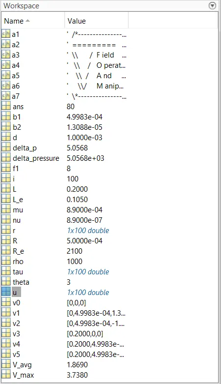
In the above code, we calculated the analytical results of the physical properties e.g - pressure, velocity, shear stress. We incorporate the values of computed pressure, velocity values in the OpenFoam.
the pressure difference = 5.056766400000001 `((kg*(sec^2))/m) / ((kg)/(m^3))` which is 5.056766400000001 `m^2*(s^2)`
since OpenFoam takes the values of pressure as pressure/density format.
average velocity = 1.8690 metre/sec.
maximum velocity = 3.7380 metre/sec.
the code for the pressure and velocity profile is as follows :
/*--------------------------------*- C++ -*----------------------------------*
  =========                 |
        /  F ield         | OpenFOAM: The Open Source CFD Toolbox
       /   O peration     | Website:  https://openfoam.org
      /    A nd           | Version:  9
     /     M anipulation  |
*---------------------------------------------------------------------------*/
FoamFile
{
    format      ascii;
    class       volScalarField;
    object      p;
}
// * * * * * * * * * * * * * * * * * * * * * * * * * * * * * * * * * * * * * //

dimensions      [0 2 -2 0 0 0 0];

internalField   uniform 0;

boundaryField
{
    axis
    {
        type            empty;
    }


    wall
    {
        type            zeroGradient;

    }


    inlet
    {
        type            zeroGradient;
    }

    outlet
    {
        type            fixedValue;
        value           uniform 5.0568;
    }

    wedgeFront
    {
         type           wedge;
    }


    wedgeBack
    {
         type           wedge;

    }
}


// ************************************************************************* //
velocity :
/*--------------------------------*- C++ -*----------------------------------*
  =========                 |
        /  F ield         | OpenFOAM: The Open Source CFD Toolbox
       /   O peration     | Website:  https://openfoam.org
      /    A nd           | Version:  9
     /     M anipulation  |
*---------------------------------------------------------------------------*/
FoamFile
{
    format      ascii;
    class       volVectorField;
    object      U;
}
// * * * * * * * * * * * * * * * * * * * * * * * * * * * * * * * * * * * * * //

dimensions      [0 1 -1 0 0 0 0];

internalField   uniform (1.8690 0 0);

boundaryField
{
    axis
    {
        type            empty;
    }

    wall
    {
        type            fixedValue;
        value           uniform (0 0 0);
    }


    inlet
    {
        type            fixedValue;
        value           uniform (1.8690 0 0);

    }

    outlet
    {
        type            zeroGradient;
    }

    wedgeFront
    {
        type            wedge;
    }

    wedgeBack
    {
        type            wedge;
    }

}

// ************************************************************************* //
Now after setting up the initial conditions we create the mesh file by executing the 'blockMesh' command and then 'checkMesh'. This command will take the parameters set at the blockMeshDict file.
We can check the mesh generated in ParaView. Now we have to calculate the physical properties for the entire simulation for the given time frame.
The simulation time and the time step values are determined in the controlDict file as follows :
/*--------------------------------*- C++ -*----------------------------------*
  =========                 |
        /  F ield         | OpenFOAM: The Open Source CFD Toolbox
       /   O peration     | Website:  https://openfoam.org
      /    A nd           | Version:  9
     /     M anipulation  |
*---------------------------------------------------------------------------*/
FoamFile
{
    format      ascii;
    class       dictionary;
    location    "system";
    object      controlDict;
}
// * * * * * * * * * * * * * * * * * * * * * * * * * * * * * * * * * * * * * //

application     icoFoam;

startFrom       startTime;

startTime       0;

stopAt          endTime;

endTime         0.5;

deltaT          0.0001;


writeControl    timeStep;

writeInterval   20;

purgeWrite      0;

writeFormat     ascii;

writePrecision  6;

writeCompression off;

timeFormat      general;

timePrecision   6;

runTimeModifiable true;


// ************************************************************************* //
After executing the icoFoam solver we get the following set of files which has solved for the flow equation.
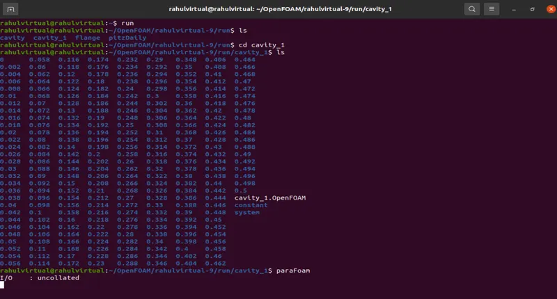
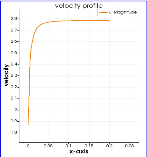
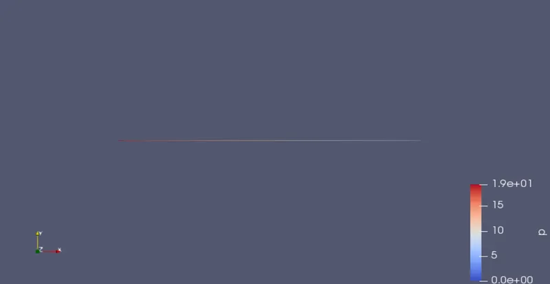
the velocity and pressure profiles look as follows :
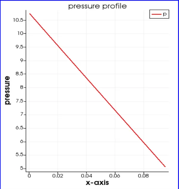
the analytical value of pressure difference is given as : 5.056766400000001
and we can see the graph the difference of the highest and the lowest value is given as follow : 10.74 - 5.0696 = 5.6704 , which is within the tolerance value.
the simulation results are as follows :
pressure :
velocity :
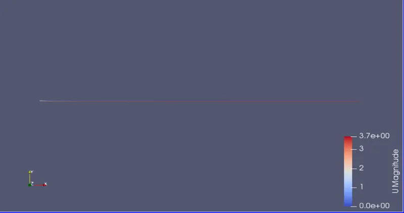
the analytical value of the maximum velocity is given as : 3.7380 metres/sec. and the value deduced by the simulation graph is given as : 2.7849 metres/sec.
the shear stress profile is also computed and plotted across the radius. the plot is as follows :
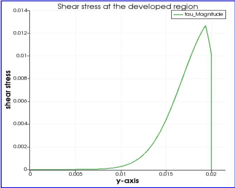
the analytical value of shear stress is maximum at the maximum radius and is given as : 13.3072800000000 `N/m^2`
the simulation graph depicts the value of shear stress as : 11.87 `N/m^2`
Hydrodynamic length : It is the length after which the velocity profile of the flow doesnt change in laminar flow cases. Hence we can see from the profile after the hydrodynamic length of 0.1050 metres the flow velocity is constant.