Simulation of a 1D Super-sonic nozzle flow simulation using Macormack Method
Aim : 1D Super-sonic nozzle flow simulation using Macormack Method.
Procedure :
The flow through the nozzle is actually two dimensional but we are only considering the x-axis direction so as to make it less complicated. We consider the grid size of n = 31 and later 61 to check the grid dependency.
At first the governing equations are defined in conservative and non-conservative form. Just that the conservative form is expressed in non-dimensional form to be converted in non-conservation form.
Defining the geometry : the C-D nozzle is given as follows
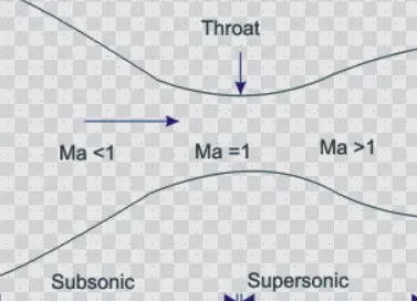
The inlet section is suppose to have area tends to infinity and the velocity is near to zero. As we progress through the nozzle the velocity increases. The inlet section is at subsonic, at the throat the speed reaches mach number = 1, and after that the throat section the mach number increases above one.
The derivation :
In the integral form of governing equation , we have control volume through which the flow passes and it is given as follows :
`del/dtintintint rho*dv + intintrho*v*ds = 0` where `rho` is density , `v` is velocity , `ds` is infinitesimial area.
`therefore d/dtintintintrho*dv = d/dtintintint(rho*A)*dx`
and the surface integral is given as inflow - outflow which is expressed as
`intintrho*v*ds = -P*V*A + (p+dp)(v+dv)(A+dA)` inflow in control area is negative according to the sign convention and the outflow is calculated by the Taylor series since we are considering a small section , the right hand side is given as : (p+dp)(v+dv)(A+dA)
After simplifying the equation the above equation we get :
`intintrho*v*ds = d(rho*A*V)`
Now we divide it dx on both sides : `d/dt(rho*A*dx) + d(rho*A*V) = 0`
`d/dt(rho*A) + d/dx(rho*A*V) = 0` ... what we get here is continuity equation.
`d/dt(rho*A*V) + d/dx(rho*A*V^2) = -A*(drho)/dx` ==== > Momentum equation.
`d/dt(rho*V^2)/(2*A) + d/dx(rho*v^3/2*(A)) = -A*V*(drho)/dx` ==== > Energy equation.
the non-conservative form is given as follows :
`d/dt(rho*A) + V*d/dx(rho*A) = -rho*A*(dv)/dx` ==== > continuity equation
`rho* (dv)/dt + rho*V*(dv)/dx = -(drho)/dx` ==== > Momentum equation
`rho*(de)/dt + rho*v(de)/dx = -rho*(dv)/dx - rho*v*d(ln A)/dx` ==== > Energy equation
the difference in both forms to note here is that in conservative form we use local derivative and in non-conservative we use substantial derivative for density. It is because, in conservative the control volume is fixed in position and in other the control volume is moving.
After figuring out the governing equations to solve , we will now jump into the Maccormack's method to solve them.
We define the grid size , no. of timesteps, initialize the primitive variables and also define the value of timestep we according to the CFL condition.
then we define the conservative and non-conservative equations in seperate functions which is user defined. Since it is a nozzle, the area of it is defined by an equation : `a = 1+2.2*(x-1.5)^2` then we define the initial density and temperature values as per the length of the nozzle.
Now we start with our time loop, in conservative form the solution for the primitive variables are not directly concluded, we first find the solution, flux and source vectors and then find the primitive variables.
The Maccormack's method involves stages as follows :
Predictor step : where we find the derivative of the equation using discretization technique and perform forward differencing on the space terms.
`(df)/dt_p`
Solution update : Here we update the predictor step by multiplying with dt and adding with the initial function value.
`f_(i nitial) + (df)/dt_p*dt`
Corrector step : here we differentiate the solution update. the exception is that here we use backward differencing on the space terms.
Averaging step : Here we find the average value of the predictor and corrector step functions.
The boundary conditions are applied at the end and time marching solution is continued till the predefined number of timesteps is reached.
Coding :
the main code of the project is as follows :
clc
close all
clear all

% inputs
n = 31;
x = linspace(0,3,n);
dx = x(2) - x(1);
gamma = 1.4;
nt = 1400;
C = 0.5
rho = zeros(1,n);
t = zeros(1,n);

a = 1+2.2*(x-1.5).^2;
v = 0.59./(rho.*a);
%dt = min(abs((C*dx)./(sqrt(t+v))));


% conservative form calculation

[u1,u2,u3,rho_c,v_c,t_c,p_c,mfr,rho_th,t_th,p_th,mach_th,mfr_th,net_mass_flow,mach,dt_c] = conserv(x,rho,t,a,v);
time = nt*dt_c;
time_c = linspace(0,dt_c,31);

figure(1)
subplot(4,1,1);
plot(time_c,rho_c);
xlabel('x-axis');
ylabel('density');
title('variation of quantities against time - conservative form')

hold on;
subplot(4,1,2);
plot(time_c,v_c);
xlabel('x-axis');
ylabel('velocity');
subplot(4,1,3);
plot(time_c,t_c);
xlabel('x-axis');
ylabel('temperature');
subplot(4,1,4);
plot(time_c,p_c);
xlabel('x-axis');
ylabel('pressure');


% non-conservative form calculation

[drhodt,dvdt,dtdt,rho_n,v_n,t_n,p_n,n_rho_th,n_t_th,n_p_th,n_mach_th,n_mfr_th,dt_n,mfr_n] = non_conserv(x,rho,t,a,v);
time = nt*dt_n;
time_n = linspace(0,time,31);

figure(2);
subplot(4,1,1);
plot(time_n,rho_n);
xlabel('x-axis');
ylabel('density');
title('variation of quantities against time - non-conservative form');

subplot(4,1,2);
plot(time_n,v_n);
xlabel('x-axis');
ylabel('velocity');
subplot(4,1,3);
plot(time_n,t_n);
xlabel('x-axis');
ylabel('temperature');
subplot(4,1,4);
plot(time_n,p_n);
xlabel('x-axis');
ylabel('pressure');

% plotting for the primitive  variables w.r.t time
k = 1400;
tt = linspace(0,k,k);

figure(3)
subplot(4,1,1);
plot(tt,rho_th);
hold on;
plot(tt,n_rho_th);
xlabel('time');
ylabel('density');
legend('conservative','non-conservative');
title('plotting for primitive variables w.r.t time')

subplot(4,1,2)
plot(tt,t_th);
hold on;
plot(tt,n_t_th);
xlabel('time');
ylabel('temperature');
legend('conservative','non-conservative');

subplot(4,1,3);
plot(tt,p_th);
hold on;
plot(tt,n_p_th);
xlabel('time');
ylabel('pressure');
legend('conservative','non-conservative');

subplot(4,1,4);
plot(tt,mach_th);
hold on;
plot(tt,n_mach_th);
xlabel('time');
ylabel('mach number');
legend('conservative','non-conservative');

% plotting mass flow rate at the throat for both.
figure(4)
plot(tt,mfr_th)
xlabel('time')
ylabel('mass flow rate')
hold on
plot(tt,n_mfr_th)
xlabel('time')
ylabel('mass flow rate')
legend('conservative','non-conservative')
title('mass flow rate for both at throat')
the function for the conservative and non-conservative form is as follows :
function [u1,u2,u3,rho_c,v_c,t_c,p_c,mfr,rho_th,t_th,p_th,mach_th,mfr_th,net_mass_flow,mach,dt_c] = conserv(x,rho_c,t_c,a,v_c)
% inputs
n = 31;
x = linspace(0,3,n);
dx = x(2) - x(1);
gamma = 2.4
nt = 1400
C = 0.5


 for i = 1:n;
       if (x(i)>=0 && x(i)<=0.5)
          rho(i) = 1
          t(i) = 1

       elseif (x(i)>=0.5 && x(i)<=1.5)
               rho(i) = 1-0.366*(x(i)-0.5)
               t(i) = 1-0.167*(x(i)-0.5)

       elseif (x(i)>=1.5 && x(i)<=3.5)
              rho(i) = 0.634-0.3879*(x(i)-1.5)
              t(i) = 0.833-0.3507*(x(i)-1.5)
       end
 end

a = 1+2.2*(x-1.5).^2;
v = 0.59./(rho.*a);
throat = find(a==1);

u1 = rho.*a
u2 = rho.*a.*v
u3 = rho.*a.*((t/(gamma-1)) + ((gamma/2)*v.^2))

for k = 1:nt
    u1_old = u1;
    u2_old = u2;
    u3_old = u3;

    dt_c = min(abs((C*dx)./(sqrt(t+v))));

    f1 = u2;
    unit1 = u2.^2./u1;
    unit2 = (gamma-1)/gamma;
    unit3 = u3-((gamma/2)*unit1);
    f2 = unit1 + (unit2)*(unit3);
    %f2 = (u2.^2./u1) + ((gamma-1)/gamma).*(u3-((gamma/2)*(u2.^2./u1)));

    beta1 = gamma*((u2.*u3)./u1);
    beta2 = (gamma*(gamma-1))/2;
    beta3 = (u2.^3)./(u1.^2);
    f3 = beta1 - (beta2)*(beta3);
    %f3 = gamma*((u2.*u3)./u1) - (((gamma*(gamma-1))/2).*((u2.^3)./u1.^2))

    % predictor step
    for j = 2:n-1
     % initial conditions
       dadt = (a(j+1)-a(j))/dx;

%        f1 = rho.*a.*v
%        f2 = rho.*a.*v + (1/gamma).*rho.*a
%        f3 = rho.*((t/(gamma-1)) + ((gamma/2).*v^2)).*(v.*a) + (rho.*a.*v)
%        j2 = (1/gamma)*rho*(da/dt)


%        term1 = (log(a(j+1))-log(a(j)))/dx;
%        j2 = ((gamma-1)/gamma)*(u3 - ((gamma/2)*(u2.^2./u1)*term1));


        df1dx(j) =  (f1(j+1) - f1(j))/dx;
        df2dx(j) = (f2(j+1) - f2(j))/dx;
        df3dx(j) = (f3(j+1) - f3(j))/dx;

        j2(j) = (1/gamma)*rho(j)*t(j)*(dadt);

        du1dt_p(j) = -(df1dx(j));
        du2dt_p(j) = -(df2dx(j)) + j2(j);
        du3dt_p(j) = -(df3dx(j));

    % solution update
        u1(j) = u1(j) + (du1dt_p(j))*dt_c;
        u2(j) = u2(j) + (du2dt_p(j))*dt_c;
        u3(j) = u3(j) + (du3dt_p(j))*dt_c;
    end

%     f1 = u2;
%     f2 = (u2.^2./u1) + ((gamma-1)/gamma).*(u3-((gamma/2)*(u2.^2./u1)));
%     f3 = gamma*((u2.*u3)./u1) - (((gamma*(gamma-1))/2).*((u2.^3)./u1.^2));

    f1 = u2;
    unit1 = u2.^2./u1;
    unit2 = ((gamma-1)/gamma);
    unit3 = u3-((gamma/2)*unit1);
    %f2 = (u2.^2./u1) + ((gamma-1)/gamma).*(u3-((gamma/2)*(u2.^2./u1)));
    f2 = unit1 + (unit2)*(unit3);

    beta1 = gamma*((u2.*u3)./u1);
    beta2 = (gamma*(gamma-1))/2;
    beta3 = (u2.^3)./(u1.^2);
    f3 = beta1 - (beta2)*(beta3);
    %f3 = gamma*((u2.*u3)./u1) - (((gamma*(gamma-1))/2).*((u2.^3)./u1.^2))

    rho = u1./a;
    t = (gamma - 1)*((u3./u1) - (gamma/2)*v.^2);
    v = u2./u1;


    % corrector step
    for j = 2:n-1
        dadt = (a(j)-a(j-1))/dx;
        c_df1dx(j) =  (f1(j) - f1(j-1))/dx;
        c_df2dx(j) = (f2(j) - f2(j-1))/dx;
        c_df3dx(j) = (f3(j) - f3(j-1))/dx;

        j2(j) = (1/gamma)*rho(j)*t(j)*(dadt);

        du1dt_c(j) = -c_df1dx(j);
        du2dt_c(j) = -c_df2dx(j) + j2(j);
        du3dt_c(j) = -c_df3dx(j);

    end

    % computing the average time derivative

    avg_du1dt = 0.5*(du1dt_p + du1dt_c);
    avg_du2dt = 0.5*(du2dt_p + du2dt_c);
    avg_du3dt = 0.5*(du3dt_p + du3dt_c);


    % final solution update
    for i = 2:n-1
        u1(i) = u1_old(i) + avg_du1dt(i)*dt_c;
        u2(i) = u2_old(i) + avg_du2dt(i)*dt_c;
        u3(i) = u3_old(i) + avg_du3dt(i)*dt_c;
    end


   % apply boundary condition
   % subsonic inlet
   u1(1) = rho(1)*a(1);
   u2(1) = 2*u2(2) - u2(3);
   u3(1) = u1(1)*((t(1)/(gamma-1))+(gamma/2)*(v(1)^2));


   % supersonic outlet
   u1(n) = 2*u1(n-1) - u1(n-2);
   u2(n) = 2*u2(n-1) - u2(n-2);
   u3(n) = 2*u3(n-1) - u3(n-2);


   % primitive variables
        for i = 1:n
        rho(i) = u1(i)/a(i);
        v(i) = u2(i)/u1(i);
        t(i) = (gamma - 1)*((u3(i)/u1(i)) - (gamma/2)*v(i)^2);
        p(i) = rho(i)*t(i);
        end

   mfr_inflow = rho(1)*v(1)*a(1);
   mfr_outflow = rho(n)*v(n)*a(n);
   net_mass_flow = mfr_inflow - mfr_outflow;


rho_c = rho;
v_c = v;
t_c = t;
p_c  = p;

mfr = rho_c.*v_c.*a;
%mfr(k) = rho_c(k).*v_c(k).*a(k);
mach = v_c./sqrt(t_c);

rho_th(k) = rho_c(throat);
t_th(k) = t_c(throat);
p_th(k) = p_c(throat);
mach_th(k) = mach(throat);
mfr_th(k) = mfr(throat);


figure(5)
if (k==50)
    plot(x,mfr,'linewidth',2,'color','b')
    hold on
elseif (k==100)
    plot(x,mfr,'linewidth',2,'color','r')
    hold on
elseif (k==500)
    plot(x,mfr,'linewidth',2,'color','g')
    hold on
    xlabel('x-axis')
    ylabel('mass flow rate')
    legend('mass flow rate at 50dt','mass flow rate at 100dt','mass flow rate at 500dt')
    hold on
    title('mass flow rate at various time steps')
    hold on
end

end

end
non-conservative form :
function [drhodt,dvdt,dtdt,rho_n,v_n,t_n,p_n,n_rho_th,n_t_th,n_p_th,n_mach_th,n_mfr_th,dt_n,mfr_n] = non_conserv(x,rho,t,a,v)

% inputs
n = 31;
x = linspace(0,3,n);
dx = x(2) - x(1);
gamma = 1.4
C = 0.5
% calculate initial profiles
rho = 1-0.3146*x;
t = 1-0.2314*x;   % temperature
v = (0.1+1.09*x).*t.^0.5;
a = 1+2.2*(x-1.5).^2;  % area
throat = find(a==1);
% time steps  % need to select values acc to courant no.
nt = 1400;

% outer time loop
for k = 1:nt;

    rho_old = rho;
    v_old = v;
    t_old = t;
    dt_n = min(abs((C*dx)./(sqrt(t+v))));
    % predictor step

    for j = 2:n-1
        dvdx = (v(j+1)-v(j))/dx;
        drhodx = (rho(j+1)-rho(j))/dx;
        dtdx = (t(j+1)-t(j))/dx;
        dlogadx = (log(a(j+1))-log(a(j)))/dx;

        % continuity equation
        drhodt_p(j) = -rho(j)*dvdx - rho(j)*v(j)*dlogadx - v(j)*drhodx;

        % momentum equation
        dvdt_p(j) = -v(j)*dvdx - (1/gamma)*(dtdx + (t(j)/rho(j))*drhodx);

        % energy equation
        dtdt_p(j) = -v(j)*dtdx - (gamma -1)*t(j)*(dvdx + v(j)*dlogadx);

        % solution update
        rho(j) = rho(j) + drhodt_p(j)*dt_n;
        v(j) = v(j) + dvdt_p(j)*dt_n;
        t(j) = t(j) + dtdt_p(j)*dt_n;

    end

% corrector method

    for j = 2:n-1
        dvdx = (v(j)-v(j-1))/dx;
        drhodx = (rho(j)-rho(j-1))/dx;
        dtdx = (t(j)-t(j-1))/dx;
        dlogadx = (log(a(j))-log(a(j-1)))/dx;

        % continuity equation
        drhodt_c(j) = -rho(j)*dvdx - rho(j)*v(j)*dlogadx - v(j)*drhodx;

        % momentum equation
        dvdt_c(j) = -v(j)*dvdx - (1/gamma)*(dtdx + (t(j)/rho(j))*drhodx);

        % energy equation
        dtdt_c(j) = -v(j)*dtdx - (gamma -1)*t(j)*(dvdx + v(j)*dlogadx);

    end

% computing the average time derivative

    drhodt = 0.5*(drhodt_c + drhodt_p);
    dvdt = 0.5*(dvdt_c + dvdt_p);
    dtdt = 0.5*(dtdt_p + dtdt_c);

% final solution update

    for i = 2:n-1
        rho(i) = rho_old(i) + drhodt(i)*dt_n;
        v(i) = v_old(i) + dvdt(i)*dt_n;
        t(i) = t_old(i) + dtdt(i)*dt_n;
    end

    % apply the boundry conditions
    % inlet
    v(1) = 2*v(2) - v(3);

    %  outlet
    v(n) = 2*v(n-1) - v(n-2);
    rho(n) = 2*rho(n-1) - rho(n-2);
    t(n) = 2*t(n-1) - t(n-2);
    p = rho.*t


rho_n = rho
v_n = v
t_n = t
p_n = p
mach_n = v_n./sqrt(t_n);
mfr_n = rho_n.*v_n.*a;

% calculation the throat values
n_rho_th(k) = rho_n(throat);
n_t_th(k) = t_n(throat);
n_p_th(k) = p_n(throat);
n_mach_th(k) = mach_n(throat);
n_mfr_th(k) = mfr_n(throat);

figure(5)
if (k==50)
    plot(x,mfr_n,'color','b')
    hold on
elseif (k==100)
    plot(x,mfr_n,'color','r')
    hold on
elseif (k==500)
    plot(x,mfr_n,'color','g')
    hold on
    legend('mass flow rate at 50dt','mass flow rate at 100dt','mass flow rate at 500dt')
    hold on
    title('mass flow rate at various time steps')
    hold on
end

end

end
Which form is better?
In terms of programming , the non-conservative form is convenient as we directly compute the primitive variables. But in conservative form the equations are expressed in flux and solution variables and then they are used to solve for the primitive variables. Also since we are directly solving the primitive variables in Non-conservative form , the results are accurate. The increased number of calculations in conservative form contributes to the rounding off of the decimals to the machine precision and that will lead to more errors.
The convergence time for the non-conservative form is shorter than the conservative.
In terms of stability only the conservative form is coming at limelight. In CFD , while solving the Governing equations we tend to encounter discontinuities. The primitive variables jump across these discontinuities. In conservative form the flux variables remains constant.
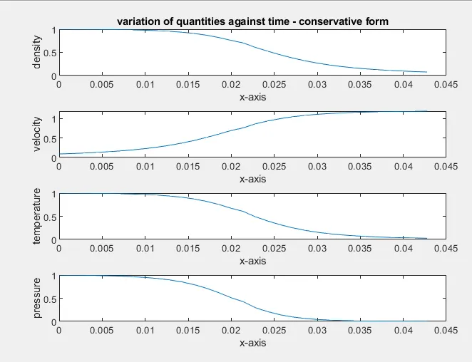
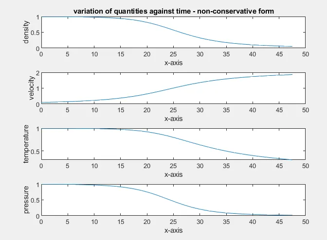
By the above graph we can conclude that there is only difference in the way we program both the forms. The primitive variables can be deduced by both the forms.
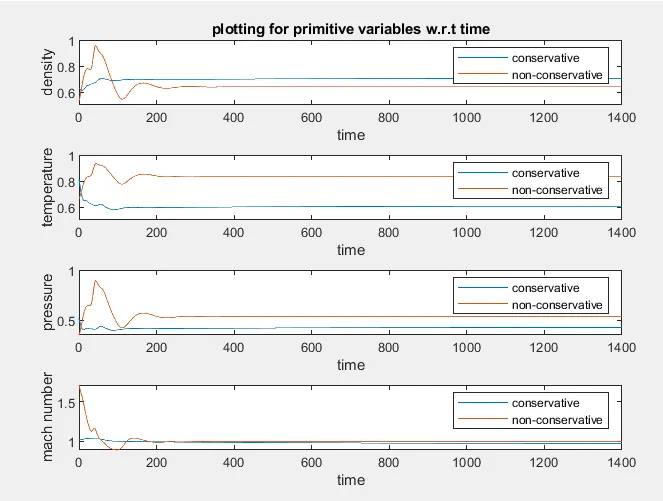
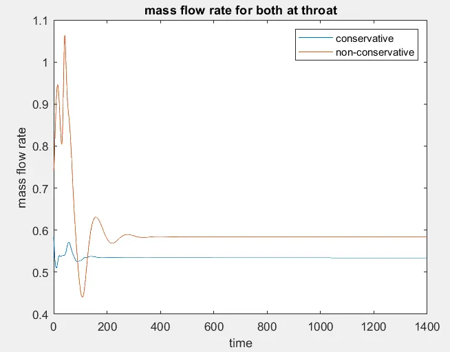
At throat , approximately at n = 16, the flow reaches mach number = 1. The above graph shows the mass flow rate at throat.
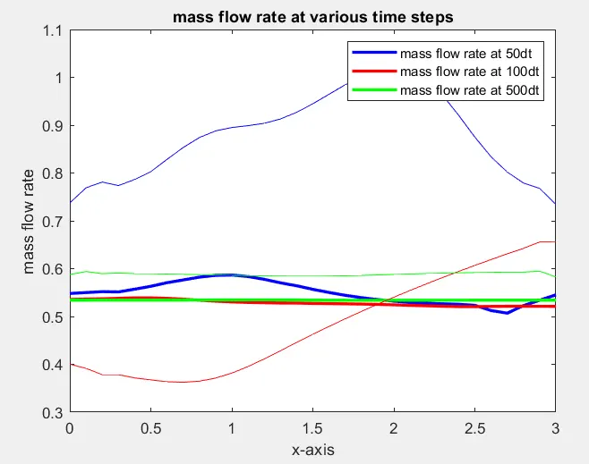
The bold lines are representing the Conservative form and the other ones are Non-conservative form. Here we can observe the mass flow rate at various timesteps.
Grid Independency test :
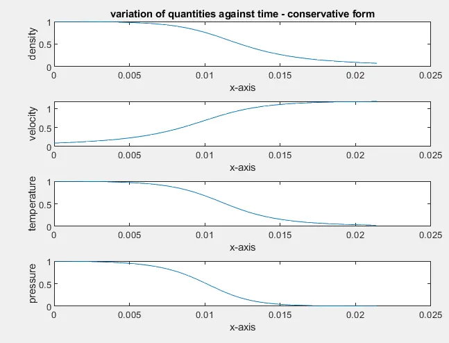
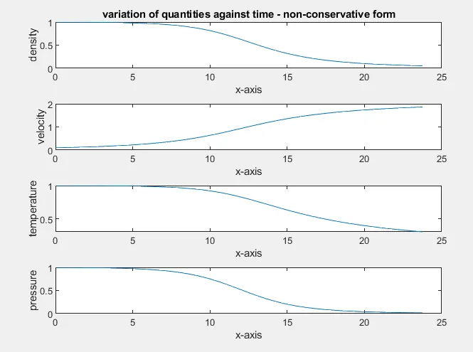
The no. of grid nodes is increased to n = 61 and checked if there is any effect on the primitive variables. In the following graph it shows that it is independent of the grid size and shows the same result as for at n = 31.
==================================== end =======================================