SIMULATING CONSERVATIVE AND NON CONSERVATIVE FORMS OF GOVERNING EQUATIONS FOR A 1D SUPERSONIC NOZZLE FLOW USING MACCORMACK TECHNIQUE
Aim : To derive the conservative and non conservative forms of governing equation for a 1D supersonic nozzle flow and simulating the flow using Maccormack technique in Matlab.
Introduction to 1D supersonic nozzle flow :
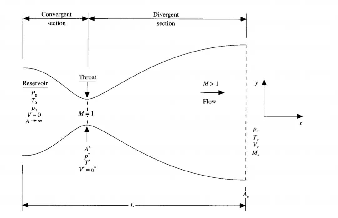
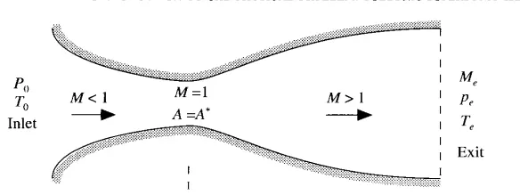
Considering a steady,isentropic flow through a convergent-divergent nozzle .The flow at the inlet to the nozzle comes from a reservoir where the pressure and temperature are denoted by Po and To, respectively.The c/s area of reservoir is large (A-->infinite) and hence the velocity is very small (V--->0).
Po and To are stagnation values ,or total pressure and total temperature respectively. The flow expands isentropically to supersonic speeds at the nozzle exit, where the exit pressure, temperature, velocity and Mach number are donoted by Pe,Te,Ve and Me, respectively. The flow is locally subsonic in the convergent section of the nozzle, sonic at the throat (M=1) and supersonic at the divergent section.
At the throat sonic means the
local velocity = local speed of sound
At throat v=v*=a*, p=p* and T=T*
Assumption :
Althought the area of the nozzle changes as a function of distance along the nozzle ,x, and therefore in reality the flow field is two dimensional (the flow varies in the 2d xy space ) the assumption is made that flow properties vary only with x, i.e uniform flow properties across any given cross section. such flow is defines as Quasi 1D flow.
The governing equations for quasi 1D flow can be expressed as
continuity : ρ1V1A1=ρ2V2A2
Momentum equation : P1A1 + ρ1A1V12 + ∫ PdA = P2A2 + P2A2V22
Energy equation : h1 + V12 /2 = h2 + V22 /2
where 1 and 2 indicate different locations along the nozzle
Perfect gas equation : P=ρRT and h = CpT
The Mach no (M) variation through the nozzle is governed by the area ratio A/A* through the relation
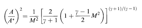
γ = ratio of specific heats
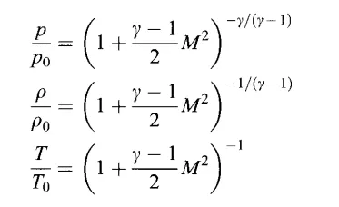
similarly the relation between pressure ratio, density ratio and temperature ratio in terms of γ and M is defined.
The governing flow equations will be couched in the form of partial differential equations suitable for the time marching solution of Quasi one dimensional flow.
Taking a control volume and deriving the equations we get the equations as follows
Dimensional Non conservative governing equations :
continuty :

Momentum equation :
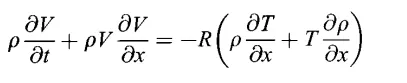
Energy equation :

These equations are in dimensional form and for the engineering advantage the equations are converted to non dimensional form .
STUDY 1 :
Non dimensional Non conservative governing equations :
continuty :

Momentum :
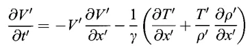
Energy equation :

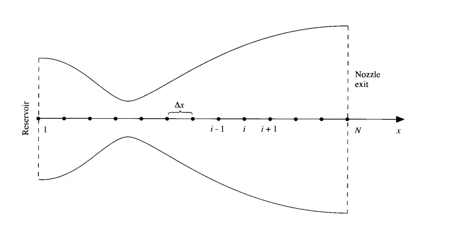
1D mesh and grid points distribution
Boundary conditions
Sub sonic inflow boundary :
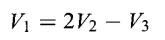

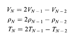
Supersonic sonic outflow boundary :
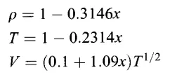
Initial conditions i.e (at t=0) :

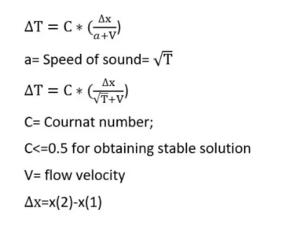
Time step calculation :
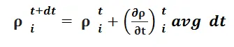
Calculation of flow variable properties at the next time step using Maccormack technique :
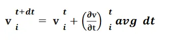
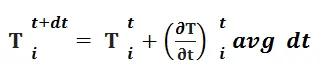



Discretization :






Necessity of conservative form :
- In the conservative form of NS equations, the variables that are being differentiated does not exist as coefficients of any derivative in the equation.on the other hand, the non-conservative form has its differentiated variables as coefficients of some derivatives in the equation.The first difference that can be noticed between both forms is in the time derivative term. The local derivative in the conservation form is replaced with a substantial derivative in the non-conservation. In the conservation form, we make the derivation under the assumption that the control volume is fixed.
- The conservative form is preferred over the non-conservative form, when the equations are being solved numerically. NS equations in the conservative form are linear differential equations (i.e. all the coefficients of the derivatives are constants), this makes the numerical scheme simpler. The non conservative form requires linearization first.
- Conservative form has an advantage, its integral form allows discontinuous solutions where as Non-conservative form does not have such a character (it allows only smooth differentiable solutions).
- So, if the governing equations are expressed in terms of flux variables (like in conservation form), irrespective of the gradients existing in primitive variables, the solution will not blow up since flux variables are the dependent variables here. Therefore, the conservation form offers better stability as compared to the non-conservation form.
- one form of governing equations will not work for all the problems. While the non-conservation form gives a more accurate result, the conservation form shows better conservation properties. While the former works better for shock-fitting applications, the latter works better for shock-capturing ones. Therefore, the choice of form largely depends on the nature of the problem and the critical parameters being measured.
Dimensional conservative governing equations :
continuity equation :
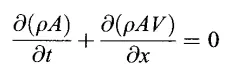
momentum equation :
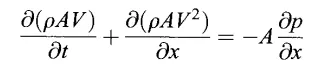
Energy equation :

These equations are in dimensional form and for the engineering advantage the equations are converted to non dimensional form.
STUDY 2:
Non dimensional conservative governing equations :
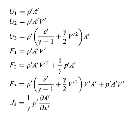
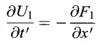
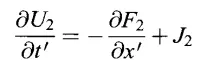
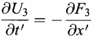
where U is solution vector F is flux vector and J is source term.
continuity equation :
momentum equation :
Energy equation :
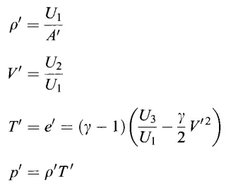
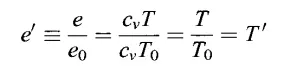
Primitive variables :
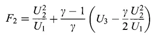
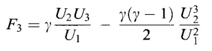
Flux variables in terms of solution vectors :

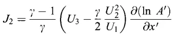
Boundary conditions
Sub sonic inflow boundary :
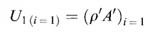

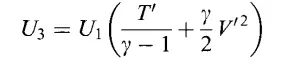
T and V are substituted at node 1
Supersonic sonic outflow boundary :
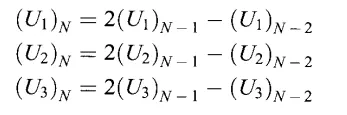
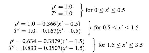
Initial conditions :
Matlab code :
%1D supersonic nozzle flow
clear all
close all
clc
%Non conservative part
%inputs
n=31;
x=linspace(0,3,n);
dx=x(2)-x(1);
nt=1400;
gamma=1.4;
%calculating the Initial profiles
rho=1-0.3146*x;
T=1-0.2314*x;
v=(0.1+1.09*x).*(T.^0.5);
a=1+2.2*(x-1.5).^2;
%calculation of minimum time step value for stability
courant=0.5;
dt=min(courant.*(dx./((T.^0.5)+v)));
tic
[x1,rho1,v1,T1,Mach1,P1,Mfr1,rho_throat1,v_throat1,T_throat1,p_throat1,Mach_throat1,Mfr_throat1]=non_conservative_maccormack(n,x,nt,dt,gamma,rho,T,v,a,dx);
t_nonconservative=toc
%conservative part
%inputs
%Initial profiles
a=1+(2.2*(x-1.5).^2); %area
for i=1:n
    if (x(i)>=0 && x(i)<=0.5)
        rho(i)=1;
        T(i)=1;
    elseif (x(i)>0.5 && x(i)<=1.5)
            rho(i)=1-0.366*(x(i)-0.5);
            T(i)=1-0.167*(x(i)-0.5);
        elseif (x(i)>1.5 && x(i)<=3.5)
                rho(i)=0.634-0.3879*(x(i)-1.5);
            T(i)=0.833-0.3507*(x(i)-1.5);
    end
end
v=0.59./(rho.*a);
%calculation of minimum time step value for stability
courant=0.5;
dt=min(courant.*(dx./((T.^0.5)+v)));
tic
[x3,rho3,v3,T3,Mach3,P3,Mfr3,rho_throat3,v_throat3,T_throat3,p_throat3,Mach_throat3,Mfr_throat3]=conservative_maccormack(n,x,nt,dt,gamma,rho,T,v,a,dx);
t_conservative=toc
ct1=1;ct2=1;ct3=1;ct4=1;ct5=1;ct6=1;
%plotting
for k=1:nt

    figure(1)
    clf
    plot(x1(k,:),v1(k,:),'r','linewidth',2)
    hold on
     plot(x3(k,:),v3(k,:),'g','linewidth',2)
    xlabel('Distance from the nozzle inlet')
    ylabel('velocity')
     axis([0 3 0 2.1])
     title('variation of velocity along nozzle length ')
     legend('maccormack non conservative','maccormack conservative','location','southeast')
     pause(0.03)
     M1(ct1)=getframe(gcf)
     ct1=ct1+1;
end
for k=1:nt
    figure(2)
    clf
    plot(x1(k,:),rho1(k,:),'r','linewidth',2)
    hold on
    plot(x3(k,:),rho3(k,:),'g','linewidth',2)
     xlabel('Distance from the nozzle inlet')
    ylabel('Density')
     axis([0 3 0 1.3])
    title('variation of density along nozzle length ')
     legend('maccormack non conservative','maccormack conservative','location','northeast')
     M2(ct2)=getframe(gcf)
     pause(0.03)
     ct2=ct2+1;
end
for k=1:nt
   figure(3)
   clf
    plot(x1(k,:),T1(k,:),'r','linewidth',2)
    hold on
     plot(x3(k,:),T3(k,:),'g','linewidth',2)
     xlabel('Distance from the nozzle inlet')
    ylabel('Temperature')
     axis([0 3 0 1.1])
    title('variation of Temperature along nozzle length ')
     legend('maccormack non conservative','maccormack conservative','location','northeast')
     M3(ct3)=getframe(gcf)
     pause(0.03)
     ct3=ct3+1;
end
for k=1:nt
     figure(4)
     clf
    plot(x1(k,:),Mach1(k,:),'r','linewidth',2)
    hold on
     plot(x3(k,:),Mach3(k,:),'g','linewidth',2)
     xlabel('Distance from the nozzle inlet')
    ylabel('Mach no')
    axis([0 3 0 3.8])
    title('variation of Mach no along nozzle length')
     legend('maccormack non conservative','maccormack conservative','location','southeast')
     M4(ct4)=getframe(gcf)
     pause(0.03)
     ct4=ct4+1;
end
for k=1:nt
     figure(5)
     clf
    plot(x1(k,:),P1(k,:),'r','linewidth',2)
    hold on
     plot(x3(k,:),P3(k,:),'g','linewidth',2)
     xlabel('Distance from the nozzle inlet')
    ylabel('pressure')
    axis([0 3 0 1.4])
    title('variation of pressure along nozzle length in non conservative part')
     legend('maccormack non conservative','maccormack conservative','location','northeast')
     M5(ct5)=getframe(gcf)
    pause(0.03)
    ct5=ct5+1;
end
for k=1:nt
     figure(6)
     clf
    plot(x1(k,:),Mfr1(k,:),'r','linewidth',2)
    hold on
     plot(x3(k,:),Mfr3(k,:),'g','linewidth',2)
     xlabel('Distance from the nozzle inlet')
    ylabel('mass flow rate')
    title('variation of mass flow rate along nozzle length')
    axis([0 3 0 2.3])
     legend('maccormack non conservative','maccormack conservative','location','northeast')
     M6(ct6)=getframe(gcf)
    pause(0.03)
    ct6=ct6+1;
end
%creating animations
movie(M1)
videofile1=VideoWriter('project1.avi','uncompressed AVI')
open(videofile1)
writeVideo(videofile1,M1)
close(videofile1)
movie(M2)
videofile2=VideoWriter('project2.avi','uncompressed AVI')
open(videofile2)
writeVideo(videofile2,M2)
close(videofile2)
movie(M3)
videofile3=VideoWriter('project3.avi','uncompressed AVI')
open(videofile3)
writeVideo(videofile3,M3)
close(videofile3)
movie(M4)
videofile4=VideoWriter('project4.avi','uncompressed AVI')
open(videofile4)
writeVideo(videofile4,M4)
close(videofile4)
movie(M5)
videofile5=VideoWriter('project5.avi','uncompressed AVI')
open(videofile5)
writeVideo(videofile5,M5)
close(videofile5)
movie(M6)
videofile6=VideoWriter('project6.avi','uncompressed AVI')
open(videofile6)
writeVideo(videofile6,M6)
close(videofile6)
%plotting at throat
 figure(7)
    subplot(5,1,1)
    plot(rho_throat1,'color','r')
    hold on
    plot(rho_throat3,'color','g')
    xlabel('Time iterations')
    ylabel('Density')
    title('variation of flow variables at throat wrt to time')
   subplot(5,1,2)
    plot(v_throat1,'r')
    hold on
    plot(v_throat3,'g')
    xlabel('Time iterations')
    ylabel('velocity ')
    subplot(5,1,3)
     plot(T_throat1,'r')
    hold on
    plot(T_throat3,'g')
    xlabel('Time iterations')
    ylabel('Temperature')
    subplot(5,1,4)
     plot(Mach_throat1,'r')
    hold on
    plot(Mach_throat3,'g')
    xlabel('Time iterations')
    ylabel('Mach no ')
    subplot(5,1,5)
     plot(p_throat1,'r')
    hold on
    plot(p_throat3,'g')
    xlabel('Time iterations')
    ylabel('pressure')
Code explanation :
1) At first nodes are defined and the inital inputs are taken
2) Minimum time step value is calculated from the corants formula.
3)The fuction codes are written seperately for conservative and non conservative forms
4) The time taken for computing is calculated for both the methods.
5) The values of the variables are calculated after 1400 time steps (i.e 1400*0.02 = 28sec) where both the forms reach their steady state values.
6) The values at the throat are also calculated in conservative and non conservative methods.
7) The function code is written such that the values of variables at all the nodes for each time step is obtained so that we can extract the values at the desired time.
8) For the conservative form initial profiles are different and are calculated again.
9) Later the variation of density, velocity , Temperature , Mach no , pressure and mass flow rate for every time step is plotted and animated.
Non conservative function code :
function [x1,rho1,v1,T1,Mach1,P1,Mfr1,rho_throat1,v_throat1,T_throat1,p_throat1,Mach_throat1,Mfr_throat1]=non_conservative_maccormack(n,x,nt,dt,gamma,rho,T,v,a,dx)
throat_node=floor(((n-1)/2)+1);
%timeloop
for k=1:nt
    rho_old=rho;
    v_old=v;
    T_old=T;
    for j=2:n-1
        %predictor step
        dv_by_dx=(v(j+1)-v(j))/dx;
        drho_by_dx=(rho(j+1)-rho(j))/dx;
        dT_by_dx=(T(j+1)-T(j))/dx;
        dloga_by_dx=(log(a(j+1))-log(a(j)))/dx;
        %continuity equation
        drho_by_dt_predictor(j)=(-rho(j)*dv_by_dx)-(rho(j)*v(j)*dloga_by_dx)-(v(j)*drho_by_dx);
        %momentum equation
        dv_by_dt_predictor(j)=(-v(j)*dv_by_dx)-((1/gamma)*((dT_by_dx)+((T(j)/rho(j))*drho_by_dx)));
        %energy equation
        dT_by_dt_predictor(j)=(-v(j)*dT_by_dx)-((gamma-1)*T(j))*(dv_by_dx+(v(j)*dloga_by_dx));

        %updating for the use of this values in corrector step
        rho(j)=rho(j)+drho_by_dt_predictor(j)*dt;
        v(j)=v(j)+dv_by_dt_predictor(j)*dt;
        T(j)=T(j)+dT_by_dt_predictor(j)*dt;
    end
    for j=2:n-1
        %corrector step
        dv_by_dx=(v(j)-v(j-1))/dx;
        drho_by_dx=(rho(j)-rho(j-1))/dx;
        dT_by_dx=(T(j)-T(j-1))/dx;
        dloga_by_dx=(log(a(j))-log(a(j-1)))/dx;
        %continuity equation
        drho_by_dt_corrector(j)=(-rho(j)*dv_by_dx)-(rho(j)*v(j)*dloga_by_dx)-(v(j)*drho_by_dx);
        %momentum equation
        dv_by_dt_corrector(j)=(-v(j)*dv_by_dx)-((1/gamma)*((dT_by_dx)+((T(j)/rho(j))*drho_by_dx)));
        %energy equation
        dT_by_dt_corrector(j)=(-v(j)*dT_by_dx)-((gamma-1)*T(j))*(dv_by_dx+(v(j)*dloga_by_dx));


    end
    %average step
    drho_by_dt_avg=0.5*(drho_by_dt_predictor+drho_by_dt_corrector);
    dv_by_dt_avg=0.5*(dv_by_dt_predictor+dv_by_dt_corrector);
    dT_by_dt_avg=0.5*(dT_by_dt_predictor+dT_by_dt_corrector);

    %calculating properties at next time step
    for i=2:n-1
        rho(i)=rho_old(i)+drho_by_dt_avg(i)*dt;
        v(i)=v_old(i)+dv_by_dt_avg(i)*dt;
        T(i)=T_old(i)+ dT_by_dt_avg(i)*dt;
    end
    %applying boundary conditions
    %inlet
    v(1)=2*v(2)-v(3);
    %outlet
    rho(n)=2*rho(n-1)-rho(n-2);
    v(n)=2*v(n-1)-v(n-2);
    T(n)=2*T(n-1)-T(n-2);

    rho1(k,:)=rho;
    v1(k,:)=v;
    T1(k,:)=T;
    P1(k,:)=rho.*T;
    Mach1(k,:)=v./(T.^0.5);
    Mfr1(k,:)=rho.*a.*v;
    x1(k,:)=x;
    %calculation of properties at throat of the nozzle
    rho_throat1(k,:)=rho1(k,throat_node);
    v_throat1(k,:)=v1(k,throat_node);
    T_throat1(k,:)=T1(k,throat_node);
    p_throat1(k,:)=P1(k,throat_node);
    Mach_throat1(k,:)=Mach1(k,throat_node);
    Mfr_throat1(k,:)=Mfr1(k,throat_node);

end
end
conservative function code :
function [x3,rho3,v3,T3,Mach3,P3,Mfr3,rho_throat3,v_throat3,T_throat3,p_throat3,Mach_throat3,Mfr_throat3]=conservative_maccormack(n,x,nt,dt,gamma,rho,T,v,a,dx)
throat_node=floor(((n-1)/2)+1);
%Defining initial solution vectors
u1=rho.*a;
u2=rho.*a.*v;
u3=u1.*((T./(gamma-1))+((gamma/2).*(v.^2)));

for k=1:nt
    u1_old=u1;
    u2_old=u2;
    u3_old=u3;
    %flux terms defined in terms of u1,u2 and u3
    f1=u2;
    f2=((u2.^2)./u1)+(((gamma-1)/gamma)*(u3-((gamma/2)*(u2.^2)./u1)));
    f3=((gamma*u2.*u3)./u1)-(gamma*(gamma-1)*(u2.^3))./(2*(u1.^2));
    %predictor step
    for j=2:n-1
        da_by_dx=(a(j+1)-a(j))/dx;
        j2=(rho(j)*T(j)*da_by_dx)/gamma;
        %continuity equation
        du1_by_dt_predictor(j)=-(f1(j+1)-f1(j))/dx;
        %momentum equation
        du2_by_dt_predictor(j)=-(f2(j+1)-f2(j))/dx + j2;
        %Energy equation
        du3_by_dt_predictor(j)=-(f3(j+1)-f3(j))/dx;
        %solution prediction
        u1(j)=u1(j)+du1_by_dt_predictor(j)*dt;
        u2(j)=u2(j)+du2_by_dt_predictor(j)*dt;
        u3(j)=u3(j)+du3_by_dt_predictor(j)*dt;
    end
  %prediction of primitives
  rho_predictor=u1./a;
  v_predictor=u2./u1;
  T_predictor=(gamma-1)*((u3./u1)-((gamma/2)*(v_predictor.^2)));
  f1=u2;
  f2=((u2.^2)./u1)+(((gamma-1)/gamma)*(u3-((gamma/2)*(u2.^2)./u1)));
  f3=((gamma*u2.*u3)./u1)-(gamma*(gamma-1)*(u2.^3))./(2*(u1.^2));
  %corrector step
  for j=2:n-1
        da_by_dx=(a(j)-a(j-1))/dx;
        j2=(rho(j)*T(j)*da_by_dx)/gamma;
        %continuity equation
        du1_by_dt_corrector(j)=-(f1(j)-f1(j-1))/dx;
        %momentum equation
        du2_by_dt_corrector(j)=-(f2(j)-f2(j-1))/dx + j2;
        %Energy equation
        du3_by_dt_corrector(j)=-(f3(j)-f3(j-1))/dx;

  end
    %average step
    du1_by_dt=0.5*(du1_by_dt_predictor+du1_by_dt_corrector);
    du2_by_dt=0.5*(du2_by_dt_predictor+du2_by_dt_corrector);
    du3_by_dt=0.5*(du3_by_dt_predictor+du3_by_dt_corrector);
    %calculating properties at next time step
    for i=2:n-1
        u1(i)=u1_old(i)+du1_by_dt(i)*dt;
        u2(i)=u2_old(i)+du2_by_dt(i)*dt;
         u3(i)=u3_old(i)+du3_by_dt(i)*dt;
    end
    %Boundary conditions
    %inlet
    u1(1)=rho_predictor(1)*a(1);
    u2(1)=2*u2(2)-u2(3);
    v_predictor(1)=u2(1)/u1(1);
    u3(1)=u1(1)*((T_predictor(1)/(gamma-1))+((gamma/2)*(v_predictor(1)^2)));
    %outlet
    u1(n)=2*u1(n-1)-u1(n-2);
    u2(n)=2*u2(n-1)-u2(n-2);
    u3(n)=2*u3(n-1)-u3(n-2);


    rho=u1./a;
  v=u2./u1;
  T=(gamma-1)*((u3./u1)-((gamma/2)*(v_predictor.^2)));
  rho3(k,:)=rho;
    v3(k,:)=v;
    T3(k,:)=T;
    P3(k,:)=rho.*T;
    Mach3(k,:)=v./(T.^0.5);
    Mfr3(k,:)=rho.*a.*v;
    x3(k,:)=x;
    %calculation of properties at throat of the nozzle
    rho_throat3(k,:)=rho3(k,throat_node);
    v_throat3(k,:)=v3(k,throat_node);
    T_throat3(k,:)=T3(k,throat_node);
    p_throat3(k,:)=P3(k,throat_node);
    Mach_throat3(k,:)=Mach3(k,throat_node);
    Mfr_throat3(k,:)=Mfr3(k,throat_node);
end

end
Animations showing variation of properties along nozzle length wrt to time:
velocity variation :
Density variation :
Temperature variation :
Mach no variation :
Pressure variation :
Mass flow rate variation :
Output :
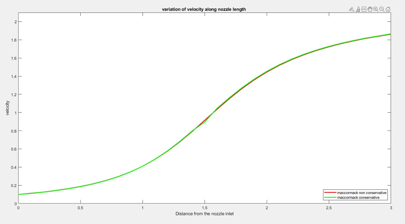
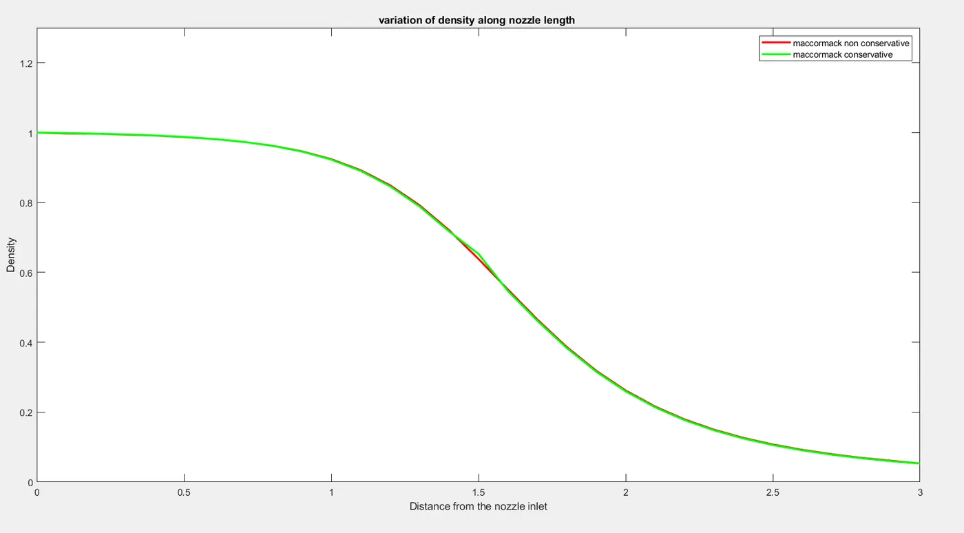
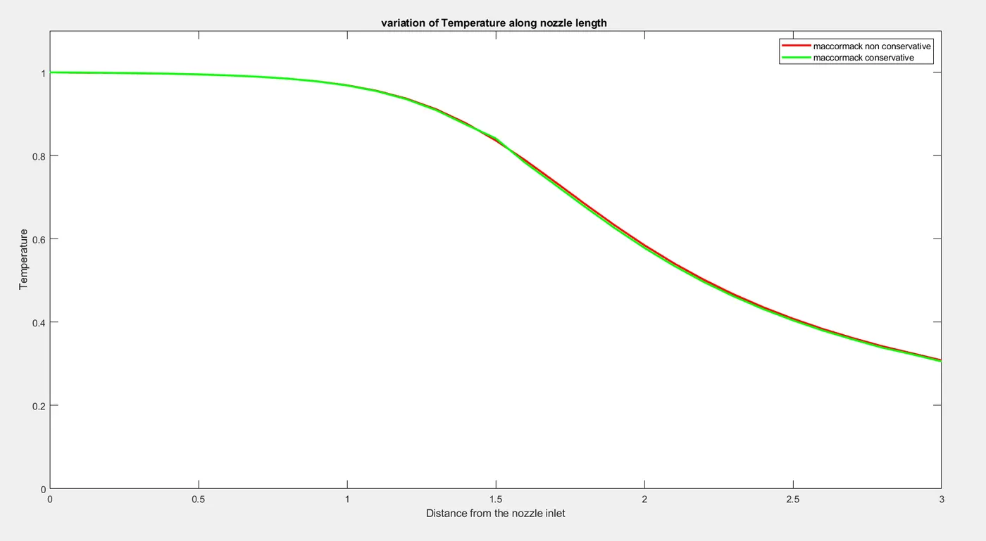
flow variables after 1400 time steps :(steady state)
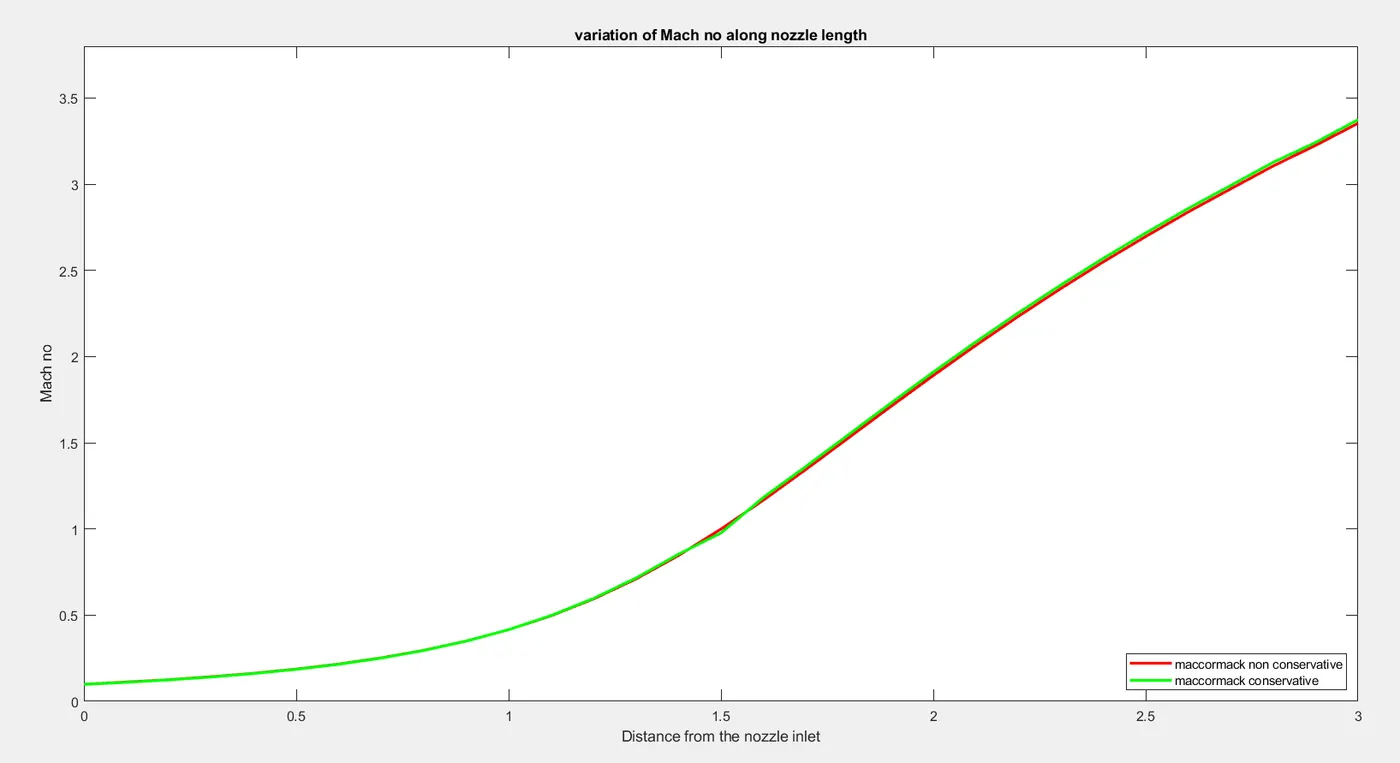
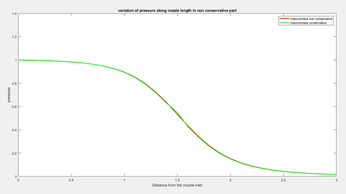
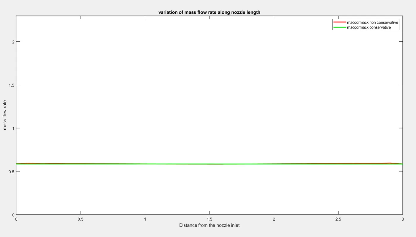
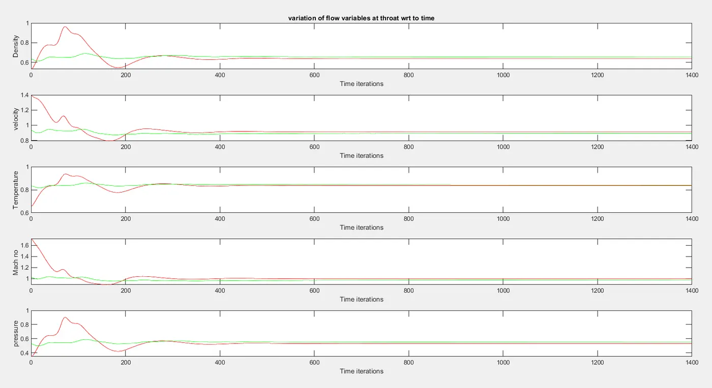
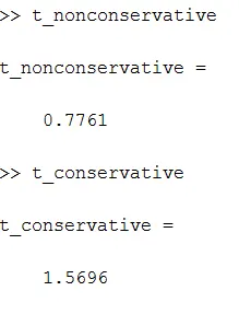
Time taken in each technique :
Flow variable values after 1400 time steps in conservative and non conservative form :
| velocity C | Velocity NC | Density C | Density NC | Temperature C | Temperature NC |
| 0.098328009 | 0.098782441 | 1 | 1 | 1 | 1 |
| 0.110280208 | 0.112004731 | 0.998742826 | 0.997798002 | 0.999512506 | 0.999114386 |
| 0.124375028 | 0.12522702 | 0.997087547 | 0.997030516 | 0.99883925 | 0.998810745 |
| 0.141094514 | 0.142610024 | 0.994859227 | 0.994274261 | 0.997963495 | 0.99770301 |
| 0.161084031 | 0.162261916 | 0.991849803 | 0.991647578 | 0.996747002 | 0.996650614 |
| 0.185121859 | 0.186553786 | 0.987691652 | 0.987338272 | 0.995096445 | 0.994915206 |
| 0.214213983 | 0.215441117 | 0.981921994 | 0.981813424 | 0.99276498 | 0.992687609 |
| 0.249556716 | 0.2507681 | 0.97380792 | 0.973782944 | 0.989508365 | 0.989433929 |
| 0.292660103 | 0.293571638 | 0.962339304 | 0.962619453 | 0.984836736 | 0.984887905 |
| 0.345240477 | 0.34578247 | 0.946014989 | 0.946662789 | 0.978164034 | 0.978335984 |
| 0.409180118 | 0.409021726 | 0.922907375 | 0.924127816 | 0.968533976 | 0.968976713 |
| 0.486155653 | 0.48503283 | 0.890559746 | 0.892490856 | 0.954811282 | 0.955613512 |
| 0.57726755 | 0.574770888 | 0.846463733 | 0.849169951 | 0.93546231 | 0.936864211 |
| 0.682056971 | 0.678011143 | 0.788758321 | 0.792061321 | 0.90910982 | 0.911268072 |
| 0.797982746 | 0.792530775 | 0.717648513 | 0.72096154 | 0.874706992 | 0.877804917 |
| 0.895603919 | 0.914013239 | 0.653238739 | 0.6386753 | 0.841427278 | 0.836454884 |
| 1.046599657 | 1.03665687 | 0.546849477 | 0.551011869 | 0.782512816 | 0.788599378 |
| 1.16420019 | 1.154611243 | 0.461675906 | 0.46496828 | 0.730182961 | 0.736798656 |
| 1.272403764 | 1.263407853 | 0.383575531 | 0.386338209 | 0.677184919 | 0.684018329 |
| 1.368785005 | 1.360586113 | 0.315942823 | 0.318366451 | 0.626111179 | 0.632829251 |
| 1.452927328 | 1.445579647 | 0.259629887 | 0.26182557 | 0.578580518 | 0.584945663 |
| 1.525524579 | 1.518961927 | 0.213898956 | 0.21591081 | 0.535365175 | 0.541262877 |
| 1.587920156 | 1.582073822 | 0.177220168 | 0.179066685 | 0.496597743 | 0.501988857 |
| 1.641455962 | 1.636180601 | 0.14796214 | 0.149649518 | 0.462121851 | 0.467018783 |
| 1.687666814 | 1.682949484 | 0.124563601 | 0.126095266 | 0.431458608 | 0.43591998 |
| 1.727483069 | 1.723106561 | 0.105812694 | 0.107208414 | 0.40438203 | 0.408398559 |
| 1.762428594 | 1.758567428 | 0.090619826 | 0.091860394 | 0.380032685 | 0.38379929 |
| 1.792478853 | 1.788681082 | 0.078302894 | 0.079476099 | 0.358875535 | 0.362106319 |
| 1.819901806 | 1.816721011 | 0.068116604 | 0.069044235 | 0.338836481 | 0.342280164 |
| 1.842477653 | 1.839256076 | 0.0597711 | 0.060953499 | 0.323013304 | 0.325280095 |
| 1.865610644 | 1.86179114 | 0.052711602 | 0.052862763 | 0.305699275 | 0.308280026 |
| Mach no C | Mach no NC | Pressure C | Pressure NC | Mass flow rate C | Mass flow rate NC |
| 0.098328009 | 0.09878244 | 1 | 1 | 0.585051652 | 0.587755526 |
| 0.110307098 | 0.11205436 | 0.998255944 | 0.996914338 | 0.585072001 | 0.593659009 |
| 0.124447275 | 0.12530155 | 0.995930177 | 0.995844793 | 0.585092351 | 0.589066649 |
| 0.141238404 | 0.14277409 | 0.992833191 | 0.991990423 | 0.58505874 | 0.59099521 |
| 0.161346675 | 0.16253434 | 0.988623318 | 0.988326168 | 0.585082004 | 0.5892401 |
| 0.185577412 | 0.1870299 | 0.982848452 | 0.982317861 | 0.585098606 | 0.589413416 |
| 0.214993135 | 0.21623316 | 0.974817769 | 0.974634021 | 0.585169834 | 0.588456932 |
| 0.250876237 | 0.25210351 | 0.963591084 | 0.963493884 | 0.585192899 | 0.588018425 |
| 0.294904501 | 0.29581534 | 0.947747099 | 0.948072256 | 0.585244428 | 0.587238166 |
| 0.349072682 | 0.34958997 | 0.925357838 | 0.926154271 | 0.585271978 | 0.5865922 |
| 0.415773776 | 0.41551787 | 0.893867149 | 0.895458333 | 0.585334791 | 0.585881949 |
| 0.497526903 | 0.49616942 | 0.850316493 | 0.852876321 | 0.585349285 | 0.585263718 |
| 0.59684835 | 0.59382221 | 0.791834919 | 0.795556936 | 0.585385982 | 0.584717644 |
| 0.715339946 | 0.71025411 | 0.717067935 | 0.721780192 | 0.585320185 | 0.584284725 |
| 0.853222308 | 0.84589631 | 0.627732172 | 0.632863584 | 0.585269896 | 0.58395466 |
| 0.976354858 | 0.99938132 | 0.549652894 | 0.534223073 | 0.585043174 | 0.583757679 |
| 1.183136515 | 1.16736539 | 0.427916725 | 0.434527617 | 0.58492379 | 0.583776865 |
| 1.362422536 | 1.34512105 | 0.33710788 | 0.342588004 | 0.584781698 | 0.584101073 |
| 1.54622007 | 1.52760018 | 0.259751565 | 0.264262416 | 0.584699413 | 0.584747066 |
| 1.729854237 | 1.71034122 | 0.197815333 | 0.201471603 | 0.584682943 | 0.585639042 |
| 1.910125883 | 1.89009774 | 0.150216795 | 0.153153732 | 0.584696206 | 0.586659058 |
| 2.084942828 | 2.06463254 | 0.114514052 | 0.116864507 | 0.584744141 | 0.587704859 |
| 2.253337741 | 2.23295364 | 0.088007135 | 0.08988948 | 0.584773048 | 0.588690573 |
| 2.414632177 | 2.39422006 | 0.068376538 | 0.069889136 | 0.584838995 | 0.589607562 |
| 2.569313753 | 2.54898742 | 0.053744038 | 0.054967446 | 0.584837201 | 0.590373683 |
| 2.716551081 | 2.69631132 | 0.042788752 | 0.043783762 | 0.584926838 | 0.591140869 |
| 2.858913764 | 2.83861793 | 0.034438496 | 0.035255954 | 0.584861581 | 0.591569356 |
| 2.992141408 | 2.97245208 | 0.028100993 | 0.028778798 | 0.585004984 | 0.59251202 |
| 3.126459986 | 3.10525574 | 0.02308039 | 0.023632472 | 0.584869371 | 0.591798146 |
| 3.241843342 | 3.22487923 | 0.01930686 | 0.01982696 | 0.584994177 | 0.595523507 |
| 3.374223195 | 3.3531908 | 0.016113898 | 0.016296534 | 0.585118983 | 0.585595574 |
Grid independence test and comparing the final results :
A CFD solution can never be trusted unless we check whether the result depends on the grid or not.or else we have any experimental data. The output result for a coarse mesh and finer mesh can never be same, so upto what extent we need to vary the mesh to get the accepted level of tolerance can be found out by the grid independence test.
This is done by varying the mesh size from coarse to fine and checking the output result for each mesh
| rho | T | P | Mach | |
| Exact analytical | 0.634 | 0.833 | 0.528 | 1 |
| NC (n=31) | 0.6387 | 0.8365 | 0.5342 | 0.9994 |
| C (n=31) | 0.6532 | 0.8414 | 0.5497 | 0.9764 |
| NC (n=61) | 0.6377 | 0.8354 | 0.5327 | 0.9998 |
| C (n=61) | 0.6392 | 0.8356 | 0.5342 | 0.9976 |
| NC(n=91) | 0.6404 | 0.8368 | 0.5359 | 1.0026 |
| C (n=91) | 0.6380 | 0.8352 | 0.5328 | 1.0004 |
Conclusion :
- From the animations the conservative solution does not vary in high amounts as compared to non conservative solutions .
- Computational time for conservative solution is more compared to non conservative form.
- From the grid independence test for the coarser nodes the non conservative form gives accurate results and when the mesh gets finer conservative form gives accurate results.
- For the conservative form the solution do not blow up where as in the non conservative form if the time step is not properly taken based on corants stability criteria the solution blows up.
References :
CFD by anderson text book