SENSITIVITY ANALYSIS FOR COMBUSTION OF METHANE FROM GRI 3.0 MECHANISM FILE USING PYTHON AND CANTERA

Aim :

To write a code from GRI mechanism for the combustion of methane and to calculate top 10 sensitive reactions wrt to temperature.

Introduction :

In any particular reaction mechanism there are multiple intermediate reactions happening which affect the rate of entire mechanism. These Reactions depend on different operating conditions and can be controlled to alter the mechanism to the desired state. In order to control the reactions we can change different conditions like temperature, pressure, species concentration etc..that have a direct impact on the rate of a particular Reaction. This impact can be studied with the help of sensitivity analysis.

Sensitivity analysis is a process of finding relationship between input parameters and the output of the system. The higher the sensitivity, greater the impact of any change in the parameter to the output.

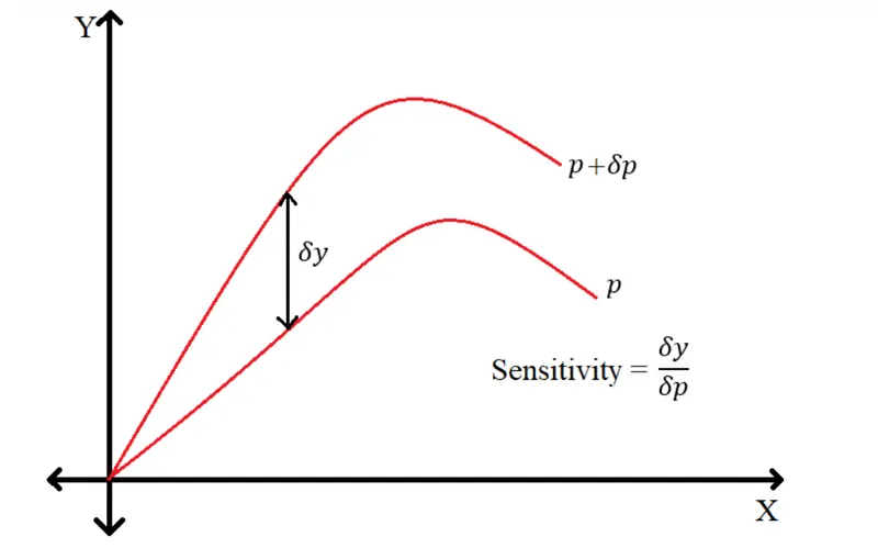
The figure represents a function `Y = f(X, p)`where `X` is an input and p is an independent parameter. The two plots represent the variation of Y when the value of p is changed from p to `p + delta p`. This change in parameter effects the value of Y by a certain value of `delta y`.Then the sensitivity of Y wrt to parameter p is defined as

Sensitivity `={delta y}/{delta p}`

Based on this sensitivity value we can adjust the value of p in order to obtain the desired value of Y Similarly for a chemical reaction mechanism there are several independent parameters that can be used to control the entire mechanism.

In this report sensitivity is calculated using cantera's inbuilt function which returns sensitivity of given parameter wrt to a reaction.

Data :

1. Initial Temperature = 1500 K
2. Initial pressure = 1atm
3. Stoichiometric mixture of CH4 and air
4. Absolute tolerance = 1e-16 (Tolerance between two iterations in a particular time step, used by cantera's solver while simulating)
5. Relative tolerance = 1e-6 (Tolerance between two time step solutions)
6. Absolute tolerance of sensitivity = 1e-6 (Absolute tolerance calculated for sensitivity)
7. Relative tolerance fot sensitivity = 1e-6 (Relative tolerance calculated for sensitivity)

Python code :

import sys
import numpy as np
import cantera as ct
import matplotlib.pyplot as plt

gas = ct.Solution('gri30.cti')
Temp=1500 # K
Press=ct.one_atm

gas.TPX=Temp,Press,{'CH4':1,'O2':2,'N2':7.52}
r=ct.IdealGasConstPressureReactor(gas)
sim=ct.ReactorNet([r])

reactions=gas.reaction_equations()   # List of all reactions in GRI file and each reaction is represented as string
no_of_reactions=gas.n_reactions      # number of reactions in GRI file 

for i in range(no_of_reactions):
	r.add_sensitivity_reaction(i)     # Adding sensitivity to each and every reaction 

max_s=[0]*no_of_reactions              # Array to store maximum sensitivity of each reaction in whole time
max_s_abs=[0]*no_of_reactions          # Array to store maximum absolute sensitivity of each reaction in whole time

sim.rtol=1e-6                       # The relative error tolerance used while integrating the reactor equations
sim.atol=1e-16                      # The absolute error tolerance used while integrating the reactor equations

sim.rtol_sensitivity=1e-6           # The relative error tolerance for sensitivity analysis 
sim.atol_sensitivity=1e-6           # The absolute error tolerance for sensitivity analysis

states=ct.SolutionArray(gas,extra='t')  # Storing solution array in states object

tot_time=2e-3
dt=5e-6

for time in np.arange(0,tot_time,dt):
	sim.advance(time)                           # Asking cantera to integrate the solution from 0 till time
	states.append(r.thermo.state,t=time*1e3)    # Saving thermodynamic state of reactor r

	for j in range(no_of_reactions):
		s=sim.sensitivity('temperature',j)   # saving sensitivity of sensitivity parameter j(i.e rxn[j]) on component(temperature)
		
		if np.abs(s)>np.abs(max_s[j]):      # Checking and saving maximum sensitivity in total time of each reaction j
			max_s[j]=s
			max_s_abs[j]=abs(s)

sen_zip=zip(max_s_abs,max_s,range(no_of_reactions))          # creating a zip data file which holds 3 variables
sen_tuple=tuple(sen_zip)                                     # converting zip to tuple in order to access the data inside the zip
sen_tuple_sorted=sorted(sen_tuple,reverse=True) # sorting the tuple based on first element of each member tupple i.e(max_abs_sens)

top_n=10                                        # Top N reactions which effect the temperature
top_rxn_index=[0]*top_n                         # Array to save index of reaction
top_rxn=[0]*top_n                               # Array to save reaction equation as string
top_sen=[0]*top_n                               # Array to save sensitivity of reaction with sign

for i in range(top_n):
	top_rxn_index[i]=int(sen_tuple_sorted[i][2])
	top_rxn[i]=reactions[top_rxn_index[i]]
	top_sen[i]=float(sen_tuple_sorted[i][1])


print("Top %d sensitive reactions for temperature are: " % (top_n))
print("---------------------------------------------------------")
print("%10s %s %18s %12s %12s" % ('Reaction Index','|','Reaction','|','sensitivity'))
print("----------------------------------------------------------")

for i in range(top_n):
	print("%7d %8s %26s %4s %10.4f" % (top_rxn_index[i],'|',top_rxn[i],'|',top_sen[i]))

print("-----------------------------------------------------------")

top_rxn_index.reverse()                   # Reversing the data in order to plot bar graph from maximum to min sensitivity
top_rxn.reverse()
top_sen.reverse()

plt.figure(1)
plt.barh(range(top_n),top_sen,0.75,align='center')
plt.yticks(range(top_n),top_rxn)
plt.xlabel('Temperature sensitivity',fontweight='bold')
plt.title('{0} most temperature sensitive reactions'.format(top_n))
plt.grid(which='major')
plt.minorticks_on()
plt.grid(which='minor',alpha=0.2)


fig1,a1=plt.subplots(2,4)

a1[0,0].plot(states.t,states.T)
a1[0,0].set_title('Temperature vs Time',fontsize=10)
a1[0,0].set_xlabel('Time in ms')
a1[0,0].set_ylabel('Temperature in K')
a1[0,0].grid('both')

a1[0,1].plot(states.t,states('CH4').X)
a1[0,1].set_title('CH4 Mole Fraction',fontsize=10)
a1[0,1].set_xlabel('Time in ms')
a1[0,1].set_ylabel('Mole fraction')
a1[0,1].grid('both')

a1[0,2].plot(states.t,states('O2').X)
a1[0,2].set_title('O2 Mole Fraction',fontsize=10)
a1[0,2].set_xlabel('Time in ms')
a1[0,2].set_ylabel('Mole fraction')
a1[0,2].grid('both')

a1[0,3].plot(states.t,states('N2').X)
a1[0,3].set_title('N2 Mole Fraction',fontsize=10)
a1[0,3].set_xlabel('Time in ms')
a1[0,3].set_ylabel('Mole fraction')
a1[0,3].grid('both')

a1[1,0].plot(states.t,states('CO2').X)
a1[1,0].set_title('CO2 Mole Fraction',fontsize=10)
a1[1,0].set_xlabel('Time in ms')
a1[1,1].set_ylabel('Mole fraction')
a1[1,0].grid('both')

a1[1,1].plot(states.t,states('H2O').X)
a1[1,1].set_title('H2O Mole Fraction',fontsize=10)
a1[1,1].set_xlabel('Time in ms')
a1[1,1].set_ylabel('Mole fraction')
a1[1,1].grid('both')

a1[1,2].plot(states.t,states('CO').X)
a1[1,2].set_title('CO Mole Fraction',fontsize=10)
a1[1,2].set_xlabel('Time in ms')
a1[1,2].set_ylabel('Mole fraction')
a1[1,2].grid('both')

a1[1,3].plot(states.t,states('OH').X)
a1[1,3].set_title('OH Mole Fraction',fontsize=10)
a1[1,3].set_xlabel('Time in ms')
a1[1,3].set_ylabel('Mole fraction')
a1[1,3].grid('both')
plt.show()

Code explanation :

1. Initial pressure, Initial temperature and mole fractions are mentioned.
2. Passing gas object to Ideal Gas Constant pressure Reactor, which is then passsed on to object r.
3. Creating a reactor network called sim by passing object r to object sim.
4. Saving all reaction equations as strings in list reactions
5. Saving the total number of reactions in mechanism file in no_of_reactions
6. Asking Cantera to compute sensitivity of reaction i while running simulation
7. Defining the Absolute and relative tolerances
8. Defining the timestep and total time for simulation
9. Advancing the solution till the total time
10. Saving the thermodynamic state of reactor object r
11. Saving the sensitivity of reaction only if it is maximum than its previous sensitivity value. Each reaction reaches a Maximum sensitivity value and then it falls. The array max_s stores the maximum values.
12. Creating a zip data variable which contains absolute and real values of sensitivities of each reaction and their index numbers.
13. Creating a tuple of Zip inorder to access the data and the members of the tuple are also a tuple which contain 3 variables.
14. Sorting the tuple using first variable of each member
15. Saving top 'n' reactions.
16. Printing the reactions
17. Reversing the reactions inorder to plot bar graphs from high sensitivity to low sensitivity.
18. Plotting the data

Results :

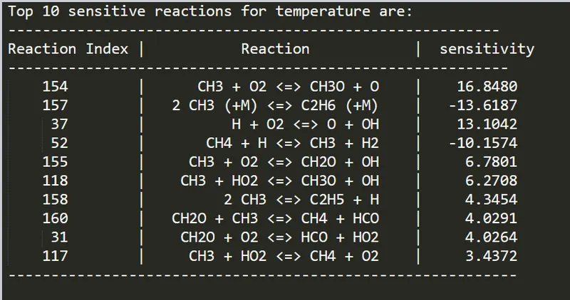
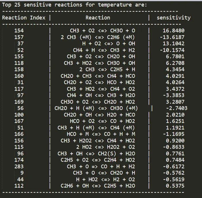
The above image lists the top 10 reactions to which the temperature is sensitive. A positive sensitivity means that increase in rate of reaction would increase temperature and negative sensitivity means that increase in rate of reaction would decrease temperature.

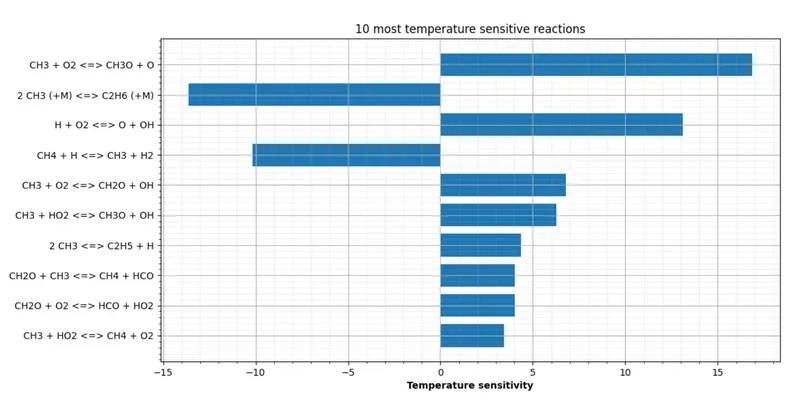
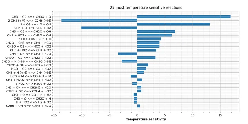
The bar graph represents temperature sensitivity wrt to top 10 reactions.

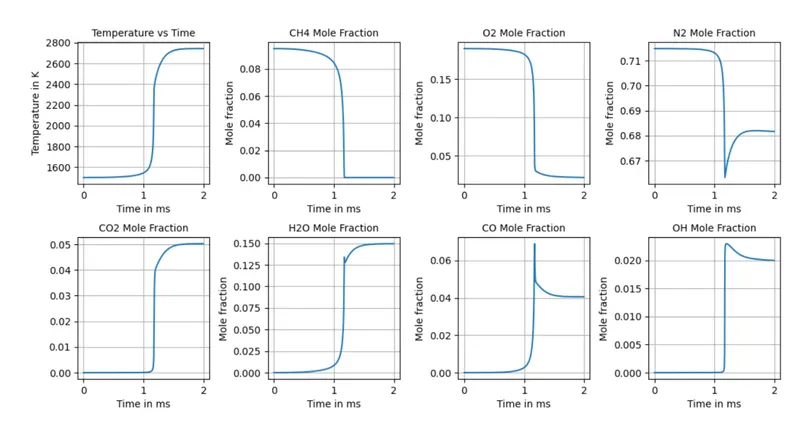
The above image shows the mole fractions of various species. The temperature is seen rising from 1500 k to 2775 k at 1.15 milli seconds. This shows that mixture is auto ignited. The CH4 concentration was seen lowering down to 0, indicating that all fuel was spent. The N2 mole fraction is seen to lower down and then rising up very little, indicating formation of NOx. Other species also show change in their molefractions.

Conclusion:

The sensitivity analysis is carried out using cantera and top 10 reactions are found which affect the temperature.