Roof crash Analysis of a car using Hypermesh and RADIOSS

AIM

The main objective of this project is to understand and carry out a Roof crash analysis of a car using Hypermesh and RADIOSS

MODEL SETUP

We open the given car model in Hyperworks desktop software by importing the starter file filename_0000.rad. We are supposed to import the FMVSS 216 Impactor which is one of the standard impactors used for Roof crash analysis. After importing both, we need to orient the impactor in a way that it is in an inclined manner above the A-pillar frame. The positioning reference is shown in the picture below.

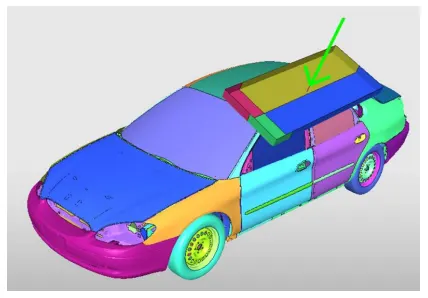
However, when the impactor is imported it is present in a random location. To orient this, a set of instructions have been given.

• A 180° rotation about the global z-axis
• A 5° rotation about the axis through axis AB
• A 25° rotation about the axis through axis AC
• A translation to put point A at global ( -3500.00, 584.822, 1343.06)

To perform these operations, we use the translate and rotate option present in the Tool menu. The points A, B and C are shown in the picture below.

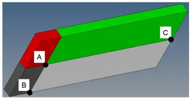
For rotation about the z-axis, the point above A is selected as the base point. For rotation about the other two axes, we use the N1, N2 and N3 option and select the corresponding points as N1 and N2. Finally, we use the translate option and enter the coordinates given in the question to bring the impactor to the expected location shown in the picture above.

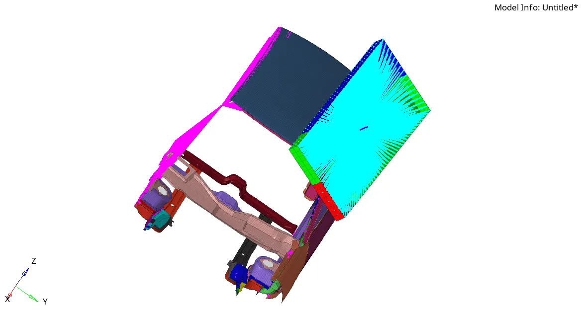
Once the impactor is placed correctly in the expected position, we proceed to the next step which is interface creation. Unlike our previous projects where we created a single contact type group(self-impact as they were explicit analyses like frontal/side crash), here we need to create two contact groups; One for self-impact as the car gets crushed and another for contact interface between the car and the impactor. We define Type 7 contact for both cases. For the self-impact case, the slave node and master surface are defined on the car alone and for the second case, the slave nodes belong to the car and the master surface is of the impactor as the mesh is coarse on the impactor and also the fact that impactor is stiffer (the reason for selecting impactor as the master surface). The recommended parameters are entered for the Type 7 contact and the values are Igap=2, Gapmin=0.5, Inacti=6, Istf=4, Stmin=1kN/mm, Idel=2, Fric=0.2 and Iform=2.

Followed by contact creation, we proceed to give Boundary conditions for the model wherever it is required. The first boundary condition is given to the three suspension shock towers. The question demands us to constrain the translation along the global z-direction. To do this, we first create a spider rigid with the nodes present on the circumference of the circle as the slave nodes and the master node is obtained by the algorithm. This can be done using 1D->Rigids. After this, we create a moving skew with the master node as the origin of the skew.

Now, we create a new BCS in the solver browser and select the master node for the node id and the newly created skew for the skew_id. Now, we tick DOF 3 which denotes the Translation along Z and DOF 6 which denotes Rotation along Z. These constraints both the degree of freedom. This procedure is repeated for all three shock towers.

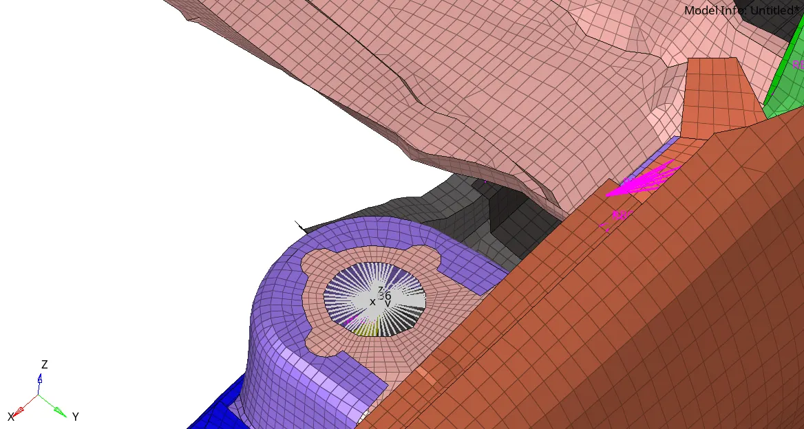
After this, we create the BCS for the free node of the spring. The condition states that the free end to be fixed in all degrees. So we create a new BCS card and select the free node and tick all the 6 boxes which constraints the node.

For the next condition, we are asked to guide the master node of the impactor rigid body so that it is free to translate in the normal direction to the face of the impactor, but is fixed in all other DOFs. To do this, we create a moving skew on the surface and make sure that the z-direction of the skew is perpendicular to the surface. Now, we create a BCS card and select the master node of the impactor rigids. Also, the skew created earlier is selected for skew_id and the constraints in all directions are selected except for the translational Z-axis (DOF 3).

Followed by this, we create a IMPDISP card for imposed displacement to the impactor. In this card, the whole impactor is selected and the direction of displacement is given as 'Z' and the skew id is selected which was given for the previous case. The displacement needs a curve for its data and now we define a curve in the model browser with two entries for time and displacement each. At t=0ms, displacement=0mm and at t=200ms, displacement =200mm. A straight line curve is created and this curve is assigned to the imposed displacement card.

With this, the initial model setup is complete. Now, we move on to the next set of instructions. Now, we are asked to check for certain control cards are present or not.

• /ANALY card
• /DEF_SHELL card,
• /DEF_SOLID card, and
• /IOFLAG card
• /SPMD card
• /TITLE card

We check the engine keywords and other keywords in the solver browser. Luckily all cards are defined already and hence we proceed to the next part where certain instructions for Engine file is given.

• Use a constant nodal time step
• Print time history every 0.0001 seconds
• Solve for 200 ms
• Create an animation file every 0.005 seconds

We check for the constant nodal time step and we observe that there's a card called DT/NODA/CST under the engine keywords which indicates constant nodal time step. After this, we change the run time to 200ms in /RUN under engine keywords. Next, to change for time history, we look for /TFILE and in that change the Time_frequency to 0.1ms(=0.0001s). Similarly, go to /ANIM/DT and change the value of Tfreq to 0.5ms(=0.0005s) to change the animation file frequency to the required value.

Now, the model setup is complete and hence we can check for the penetrations and intersections using the penetration checker. We find out that there are certain intersections/penetrations in the model.

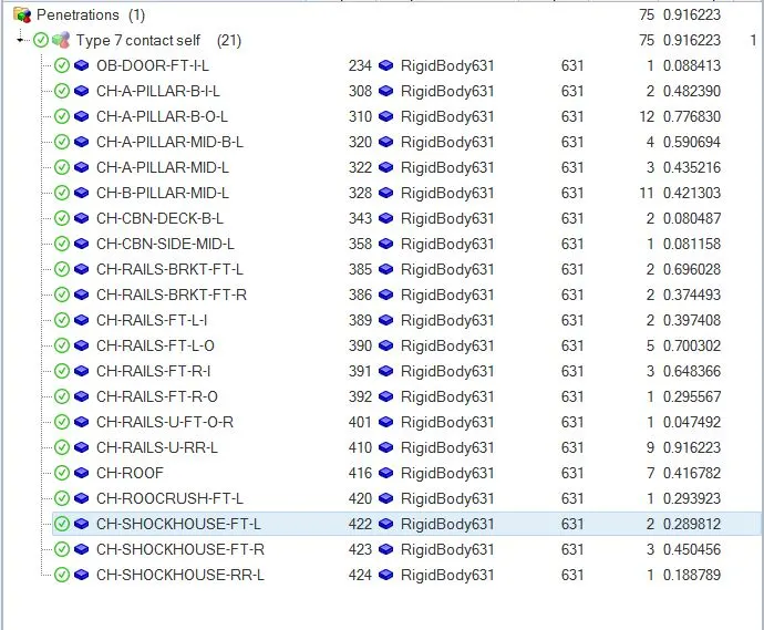
These penetrations are shown as less than 1mm and hence shown as errors. These errors are rectified and the checker is run again and made sure that no anomalies are present. After this, we run the model in the model checker and find that there are zero errors and a few warnings. Once the warnings are rectified our model is ready to run. We save the model in a new folder and run the analysis by hitting the Radioss button in the analysis bar.

OUTPUT PROCESSING

With this, we can proceed to output extraction as the model set up is complete. We take a look at the simulation time the cycles.

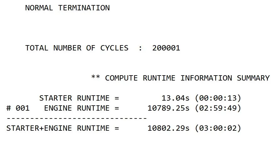
We can observe that we got the normal termination and the total number of cycles is 200001 and it took around 3 hours to complete the simulation. With this, we analyse the energy error and mass error values.

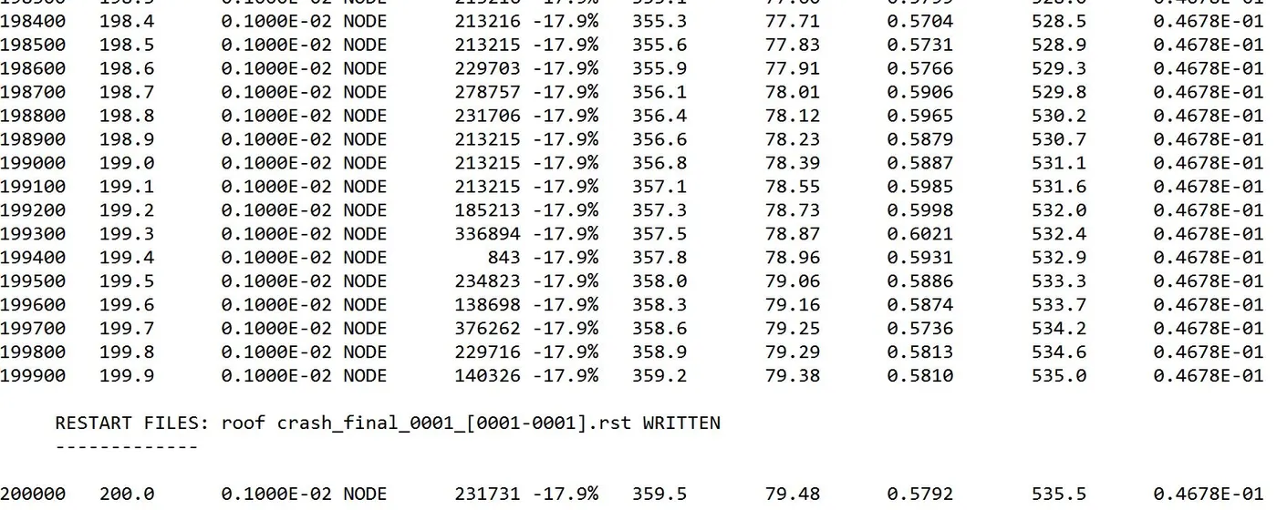
We can observe that the value of energy error is -17.9% which is a significantly large value. The reason for this can be due to nodes that are not constrained properly. The mass error is 0.046kg which is a small value and acceptable for the model. After this, we plot the different energies for the analysis.

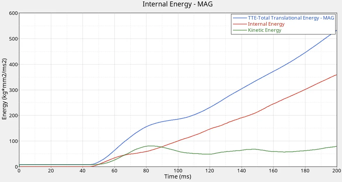
The value of potential energy is closer to 360kg*mm^2/ms^2 and the value of kinetic energy is closer to 80kg*mm^2/ms^2 which is 14% of the total energy. The reason for the lower kinetic energy is because this simulation is quasi-static one rather an explicit analysis (like frontal/side crash analysis) as the car is stationary and not moving.

Next, we take a look at the contact energy and hourglass energy.

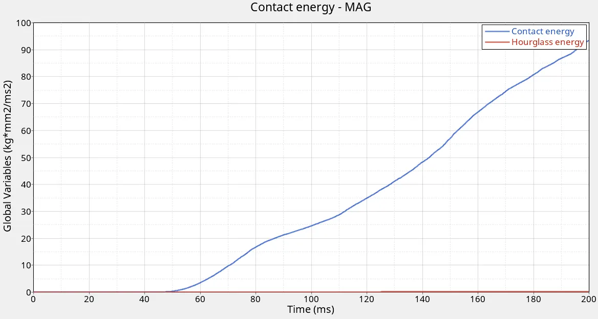
The contact energy keeps increasing gradually to a maximum value of 90kg*mm^2/ms^2 while the hourglass is very less but not zero as we would've ideally expected. The plot showing the hourglass energy is shown below.

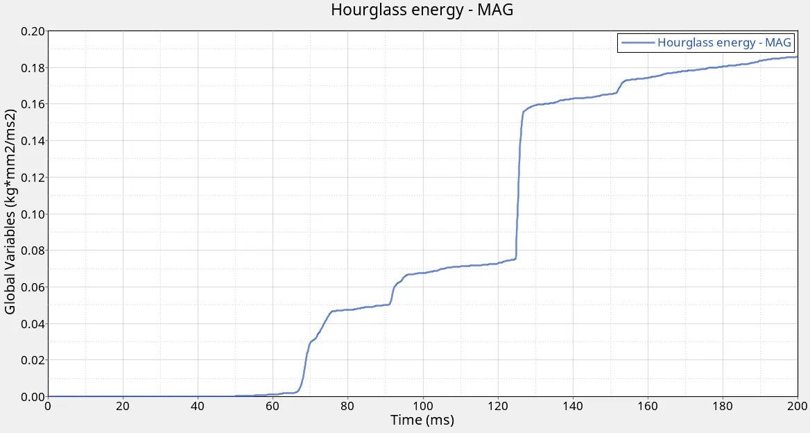
The maximum value of hourglass energy is close to 0.19kg*mm^2/ms^2 which is a negligible value. Next, we plot the forces experienced plot in the Type 7 contact.

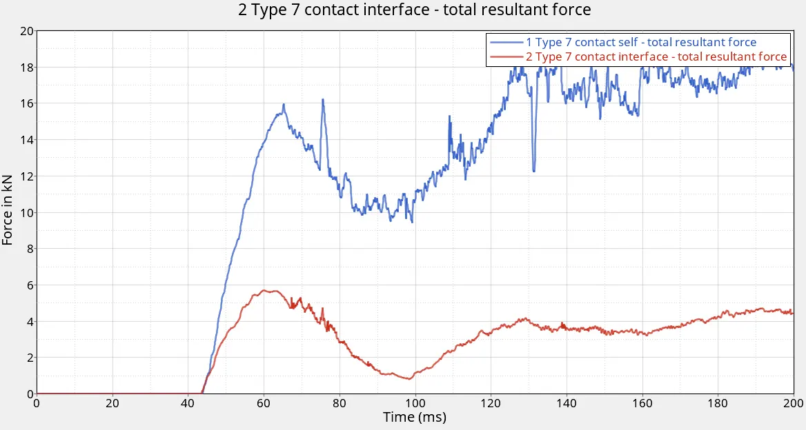
We compare the forces obtained from the two different contacts defined earlier. As expected, the force experienced in the self-impact case is higher than that of the interface between car and impactor case. In the question, we are asked to plot the Force vs displacement; However, the HyperGraph 2D plots all the parameters vs time and hence we are going to cross plot Force vs time and Displacement vs time. The Displacement vs time is plotted for a single node on the impactor which is a linear curve and the force vs time is plotted for the contact interface between car and the impactor. Then we use the math option in the menu bar, select two curves and keep displacement vs time in the x-axis and force vs time in the y-axis. This cross plots both the curves.

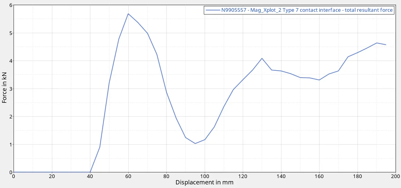
We label the axes properly and we also observe the plot containing all three plots.

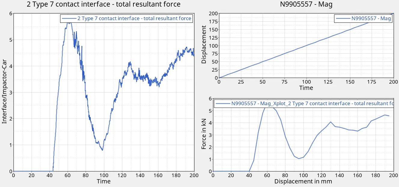
The question asks us to check for the condition where the maximum force experienced on the impactor is equal to 3 times the GVW (Gross Vehicle Weight). We don't know the gross vehicular weight as this is not the whole model but use the mass of the car model to make the calculations.

We find the mass of the car model as it is to be 175kg and this when multiplied by 3 and g(acceleration due to gravity)

Force = 175*9.81*3 = 5150.25N = 5.15kN

The maximum value of force obtained from the plot is 5.69kN which is closer to the expected value of 5.15kN which means the FMVSS crash standards are met by our model.

With this, we have completed plotting all the necessary curves required for analysis. Now, we are asked to print the animation files for certain parameters.

• Elemental Energy
• Elemental equivalent plastic strain
• Elemental von Mises stress
• Nodal added mass

To plot the contours, we open the animation file named .h3d in Hyperview and enable the contours option. This gives us various We start with the specific energy animation.

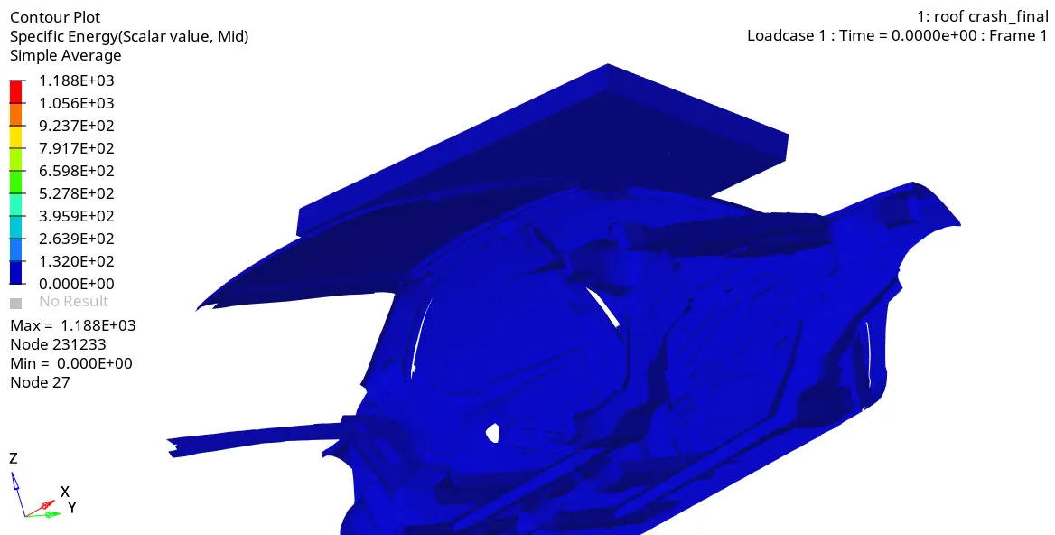
Although no visible changes in the energy can be observed, the roof of the car experiences energy change due to it getting crushed. The maximum value is 1188 units at node 231233.

Next, we print the animation for plastic strain.

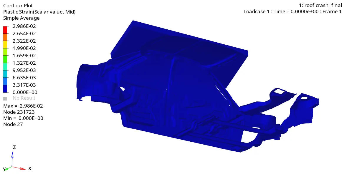
We get a small value of plastic strain and similar to the previous case it can be observed on the roof of the car and the maximum value is 0.002986 at node 231723. Followed by this, we plot the nodal added mass.

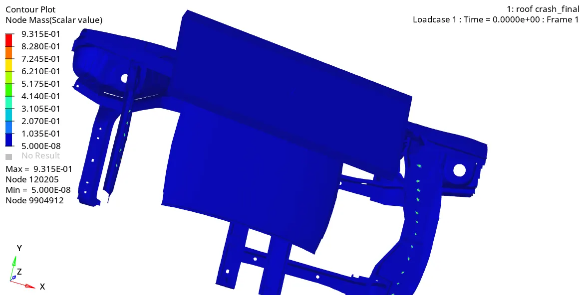
The mass added in the model is very small values primarily in the hood region and the rear bonnet region as it can be observed in the animation shown above. The final animation is printed for Von-mises stress.

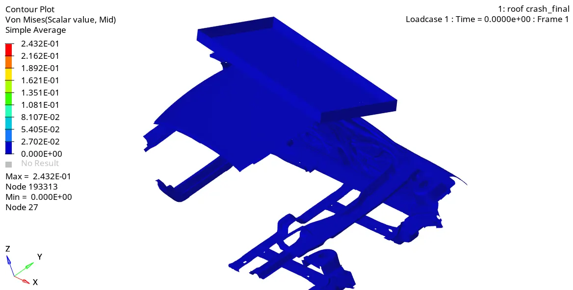
The stress propagation can be observed clearly in the animation shown above. We can observe that other than the roof, the frontal frame and parts of the frontal chassis is also affected because of the impact. The lower cross member is also affected and also the parts of the door frame along with the A-pillar and B-pillar are affected. With this we have completed the expected analysis of the model.

OBSERVATIONS AND CONCLUSION

We can observe that quasi-static analysis is also an important aspect of Crashworthiness analysis as it involves various considerations to be taken care of and standard procedure followed. In our case, we have taken FMVSS 216, Roof Crush Resistance for our analysis to test the strength requirements of the passenger compartment roof of passenger cars. This test will help in designing the roof so that it can withstand the said load acting on it and preparing for the eventuality when something wrong happens, the passengers present inside are protected.

With this, we conclude the Roof Crashworthiness Analysis.