Frontal Crashworthiness analysis of a car using Hypermesh and RADIOSS

Aim

The main objective of this project is to perform frontal crash analysis using RADIOSS in Hyperworks software after setting up the model and also processing the outputs.

Expected Setup and Requisites for the project

Model setup requests

• Check unit system and either follow[Mg mm s] or [Kg mm ms].
• Create an appropriate interface, friction 0.2 and recommended parameters.
• Make sure of no penetrations and intersection.
• Correct rigid bodies if any issues.
• Create a rigid wall with friction 0.1.
• Compare the model weight with the full-scale 300k nodes model and use added masses to reach target weight 700kg while getting CG about the required range.
• Initial velocity 35 mph.
• Use model checker to ensure good quality.
• Time-step :0.5 to 0.1 microseconds.
• Run 80 ms.

Output requests

• Sectional force in the rails at the location of indicated node 174247.
• The axial force received on the rails from the bumper.
• Shotgun cross-sectional forces.
• A pillar cross-section.
• Acceleration curve received on the accelerometer at base of B pillar (on B pillar rocker).
• Intrusions on the dash wall 66695,66244.

Model setup

Step by step procedure for setting up the model is explained below.

We start by importing the model in the Radioss format of the Hyperworks software. The same model is also opened in Hypercrash as it provides for better visualisation and understanding of the model which lacks in Hypermesh interface.

We ensure that the units are consistent throughout the model. This can be verified by checking the value of density and Young's Modulus values and cross-referencing with the consistent units provided for the solvers online.

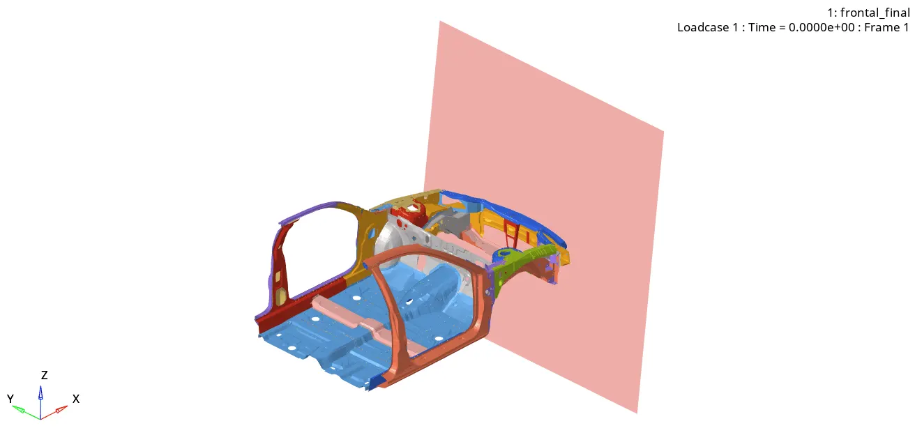
The units used by us is kg mm ms kN which stands for kilograms, millimetre, millisecond and Kilonewtons respectively. After ensuring the consistent units, we move on to the creation of Rigid wall for the analysis. For this, we use Rwall keyword in solver and select the Infinite wall as frontal crash requires a plane wall for analysis. The value of friction is taken to be 0.1. For creating the rigid wall, a point closer to the centre of the bumper is selected and the normal direction is specified properly.

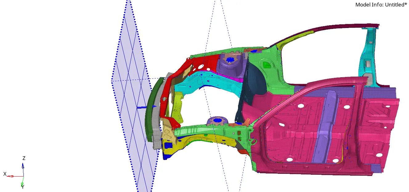
The blue plane indicates the wall along with the normal direction shown in blue vector. Followed by this, we move on to create the contact interface. There are a few contacts defined initially for other parts of the model which are of no use to our analysis and hence we delete it. Now, we use Type 7 contact which corresponds to Node to Surface contact wherein the slave nodes interact with the master surface. In our case, we select the whole component for both slave nodes and master surface as we analyse the model for self-impact. The recommended parameters' values for Type 7 contact such as Igap=2, Gapmin=0.5, Inacti=6, Istf=4, Stmin=1kN/mm, Idel=2, Fric=0.2 and Iform=2 are given.

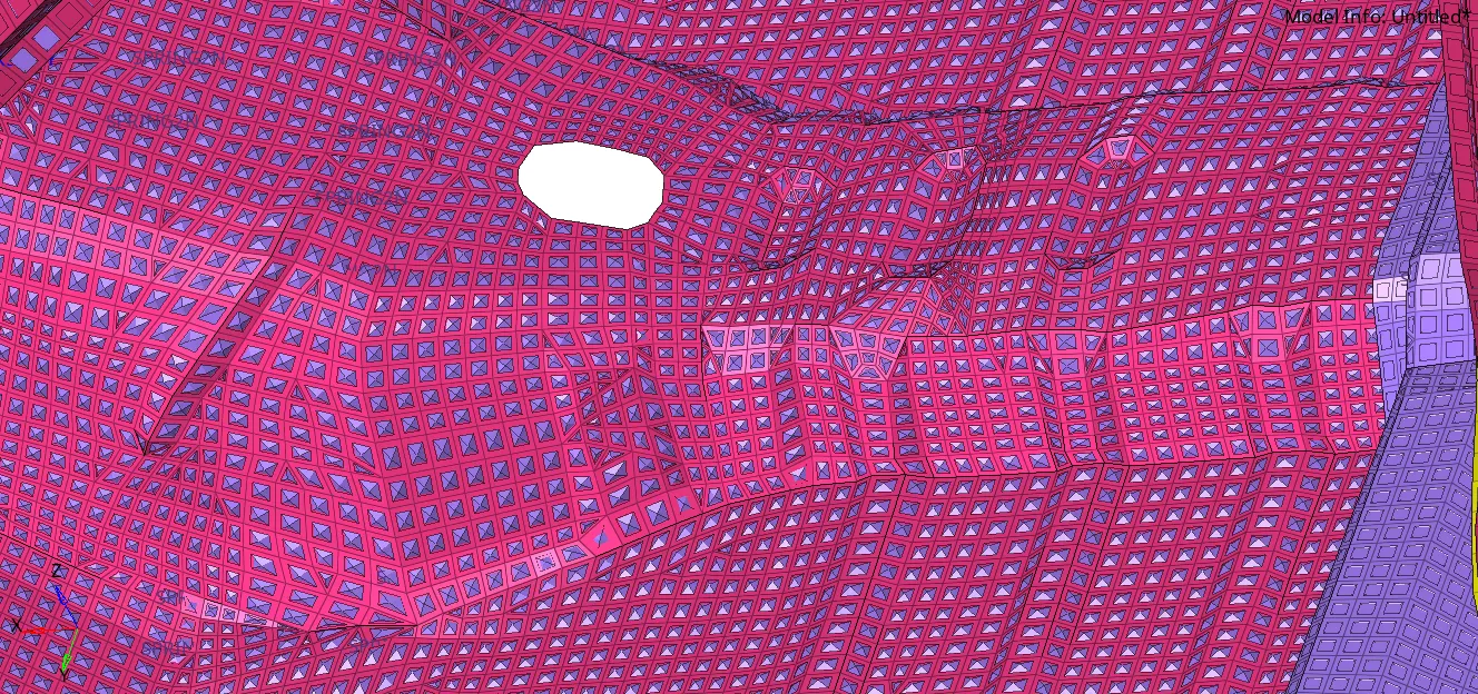
After this step, we are required to add mass to the model to achieve the target mass of 700 kg. Initially, the mass of the model is less than 200kg. So, we add 4 different types of masses in 4 different areas of the car to achieve the required mass and also move the COG of the model to the required region in the process.

The masses that are added are 132kg on the floor panel by selecting the type wherein the mass is added to a group of nodes and three 126kg added on the floor, and on either side of the car in the rear portion to pull the Center of Gravity to the region where it is supposed to be (front passenger seat of the car). These additions move the COG further behind and also achieve the target mass of 700kg.

Now, we set the initial velocity for the model. The command for this is INIVEL created in the solver; all the nodes are selected for the set and given velocity value is entered (35 mph converted to 15.65mm/ms) along the global x-direction. Now, we check for Intersections and penetrations using the Penetration checker but we find zero issues there.

Now, we are going to set up the output requirements. We start with creating sections on the required areas as we are asked to calculate the force in those regions among other parameters. Before creating a section, we need a local frame of reference to get more reliable results without uncertainty. We create a moving frame on all the required regions. It is created by selecting three nodes. The first node marks the origin, the second marks the x-direction and the third nodes define the XY-plane. While creating the section N1, N2 and N3 nodal positions are entered and the skew selected for skew_id. The sections and skews are created in the required regions mentioned below.

• Shotgun Region
• Bumper rail meeting region
• A-pillar

Also, the sections are created on either side of the symmetrical axis of the car so that the differences and variations are spotted. Followed by this, we create accelerometers on the B-pillar rocker on both sides to obtain the acceleration in this region. With this, the model is set up completely except for the output setup. For output, we create TH file which represents Time History for which the results are displayed to be plotted in the HyperGraph 2D. We use this TH for Interfaces, Accelerometers and also Sections as output is required in these regions. Also, we take TH for some nodes for which results are requested such as force and intrusions.

With this, we have set the model up and we run the model checker which displays the different errors and warnings present in the model. We fix these issues manually and also automatically (for certain ones) and completely free the model of errors so that simulation can run without any interruptions. We save the model in a new folder and run the analysis by hitting Radioss button in Analysis option.

Processing the output and results

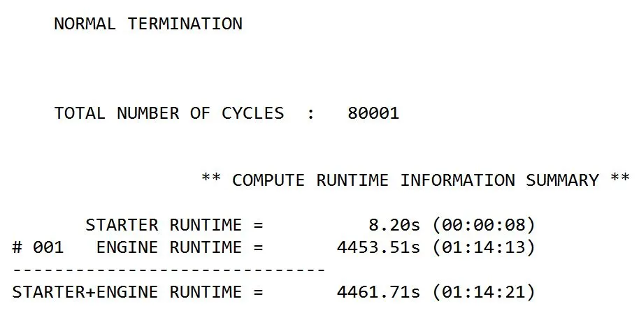
The model runs for a total time of 1 hour and 14 minutes with 80001 cycles.

We start the results processing with mass error and energy error analysis.

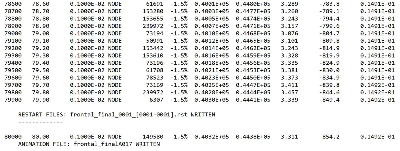
We get an energy error of -1.5% and a mass error of 0.015kg. Both these values are acceptable for simulation and hence we can say that the model has run its proper due course without much hassle.

Now, we start the outputs by plotting the energies.

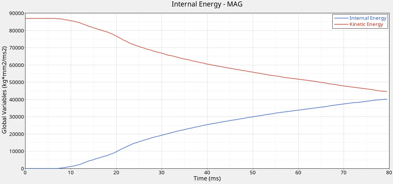
The internal energy starts at zero and the kinetic energy at the maximum and the at the end of the simulation, we values converge to a common equilibrium value of around 45000 units.

The plot for contact energy and hourglass energy is shown below.

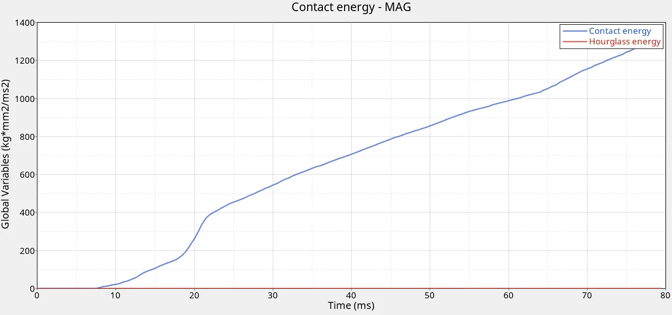
The contact energy keeps increasing after starting from zero because of the impact against the wall but the value of Hourglass energy remains zero which is a good sign.

The TTE(Total Translational Energy) is also plotted against time as this shows how energy is dissipated upon crumbling of the car.

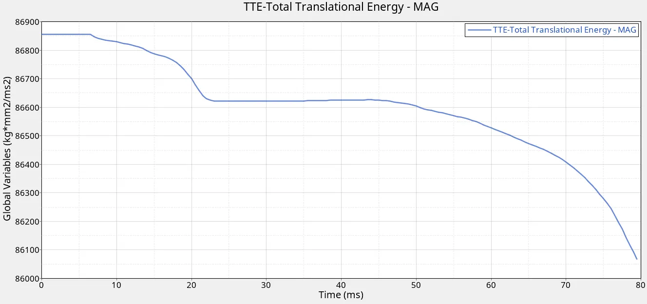
The energy starts reducing rapidly after the impact but stays constant after a certain time and this may be attributed to frontal crumple zone and starts reducing further when the car mainframe starts crumpling.

After this, we proceed to the analysis of the sectional forces.

To plot the forces, we choose HyperGraph 2D and select the T01 file which contains all the Time History files.

We start with the sectional forces for the specified node. This node is present in the rail that connects the frontal bumper to the main body. We plot the resultant force which is shown below.

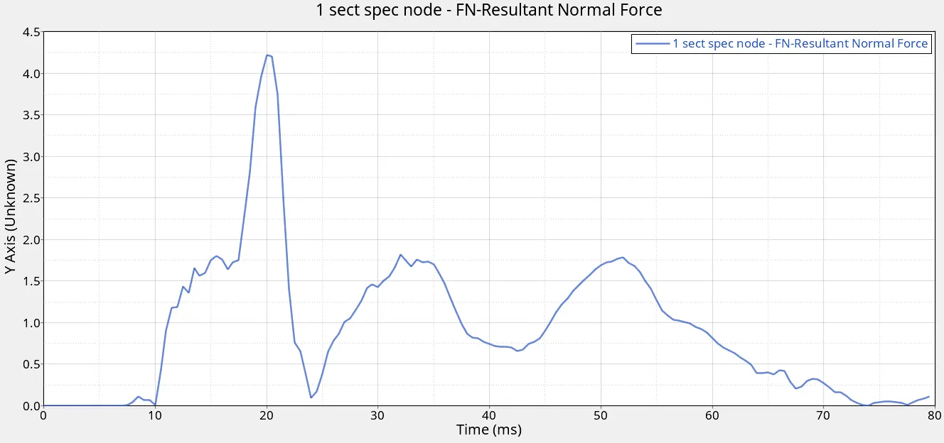
The peak value of force is around 4.25kN and it keeps fluctuating till the simulation is complete.

Followed by this, we plot the axial force received by the bumper rail. For this rail, as the axial force is requested we check the local skew frame to determine the axial direction. For the first rail section, it's in the z-direction and for the second case, it's in the x-direction.

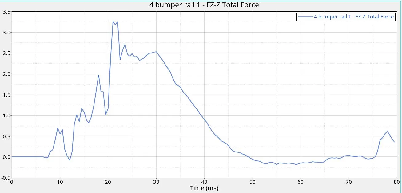
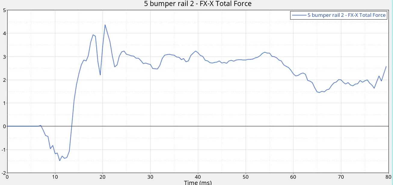
Comparing both the sides indicate that the force transmission was not identical. Also, the maximum on the left side was closer to 3.75kN and on the right, it is closer to 4.5kN.

After this, we take a look at the forces in the shotgun region. Resultant normal forces are considered as this case doesn't require a certain specific force like the previous case (axial force).

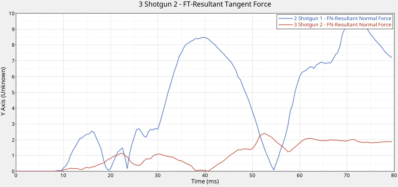
This case provides significantly varied results for both sides as one has a maximum value of 8.5 units while other has a maximum of 2.5 units. This means that the impact on one side was larger than that on the other side. This can be attributed to the added masses which might not be uniformly present on both sides.

After this, we take a look at the sectional forces in the A-pillar.

For the A-pillar, however, we obtain identical results on both the sides and according to the local skew system, the x-axis represents the axial force.

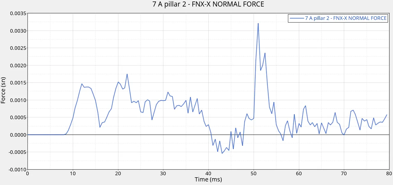
Although it fluctuates in the negative direction for a certain time, the peak value of force is in the positive direction only. The unit of the force is in Sthene system which when converted to kN gives a maximum value of 3.25kN.

The final force plot belongs to Type 7 contact to show the contact forces.

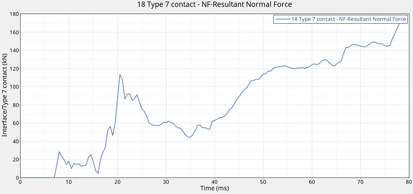
The contact force keeps increasing till the end of the simulation to a maximum value of 180kN.

With this the force analysis is complete.

Now, we observe the results for the intrusions of the two specified nodes. These two nodes with id 66695 and 66244 are present on the car's mainframe below the instrument dashboard panel. The intrusions are checked in these regions so as to make sure that the displacement is not very high as this will affect the passengers if the value is large.

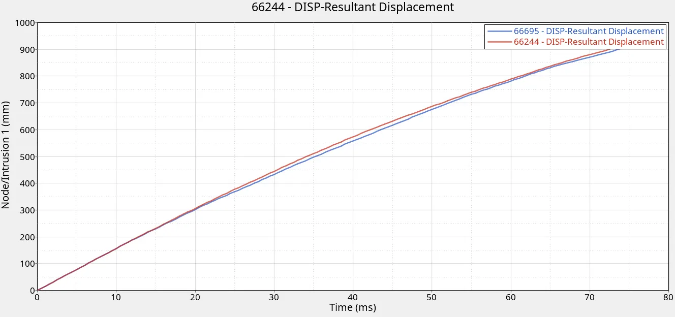
The displacement of both the nodes is almost the same (closer to 1000mm). Followed by this, we proceed to the acceleration analysis. The accelerometer placed on the B-pillar rocker on either side measures the acceleration value and the resultant acceleration is plotted here.

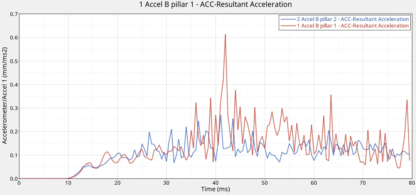
The overall maximum value of acceleration is 0.6mm/ms^2 or 600m/s^2 but the on the other side it is closer to 0.27mm/ms^2 or 270m/s^2. As we can see the plots are not similar on both sides. With this, we have obtained all the expected results requested from us in the question.

Finally, the animation file has been attached for the viewers' understanding of the crash analysis.

Observations and Conclusion

From this analysis, we can observe that frontal crash analysis is a crucial analysis in the automobile industry. Multiple factors are to be considered for the model to be set up as per the requirements. Also, we observe the effect of forces on different components of the model and how it changes the way it interacts with the other components. Energy and Forces are the most important aspects of the analysis as they require the majority of focus because this helps the engineers in analysing the behaviour of the car upon occurrence of an accident. This helps them overcome the critical issues persistent to the model in a way that doesn't cost a lot of money.

We can conclude by saying Frontal Crash is a vital part of any Crashworthiness Analysis as this forms the basis and foundation for building a car that ensures the safety and also follows safety protocols.