Rayleigh Taylor Instability Challenge

RAYLEIGH-TAYLOR INSTABILITY CHALLENGE

INTRODUCTION:

what is Rayleigh Taylor instability?

The Rayleigh–Taylor instability, or RT instability (after Lord Rayleigh and G. I. Taylor), is an instability of an interface between two fluids of different densities which occurs when the lighter fluid is pushing the heavier fluid Examples include the behavior of water suspended above oil in the gravity of Earth, mushroom clouds like those from volcanic eruptions and atmospheric nuclear explosions, supernova explosions in which expanding core gas is accelerated into denser shell gas,instabilities in plasma fusion reactors and inertial confinement fusion.

Water suspended atop oil is an everyday example of Rayleigh–Taylor instability, and it may be modeled by two completely plane-parallel layers of immiscible fluid, the more dense on top of the less dense one and both subject to the Earth's gravity. The equilibrium here is unstable to any perturbations or disturbances of the interface: if a parcel of heavier fluid is displaced downward with an equal volume of lighter fluid displaced upwards, the potential energy of the configuration is lower than the initial state. Thus the disturbance will grow and lead to a further release of potential energy, as the more dense material moves down under the (effective) gravitational field, and the less dense material is further displaced upwards. This was the set-up as studied by Lord Rayleigh. The important insight by G. I. Taylor was his realisation that this situation is equivalent to the situation when the fluids are accelerated, with the less dense fluid accelerating into the more dense fluid. This occurs deep underwater on the surface of an expanding bubble and in a nuclear explosion.

As the RT instability develops, the initial perturbations progress from a linear growth phase into a non-linear growth phase, eventually developing "plumes" flowing upwards (in the gravitational buoyancy sense) and "spikes" falling downwards. In the linear phase, the fluid movement can be closely approximated by linear equations, and the amplitude of perturbations is growing exponentially with time. In the non-linear phase, perturbation amplitude is too large for a linear approximation, and non-linear equations are required to describe fluid motions. In general, the density disparity between the fluids determines the structure of the subsequent non-linear RT instability flows (assuming other variables such as surface tension and viscosity are negligible here). The difference in the fluid densities divided by their sum is defined as the Atwood number, A. For A close to 0, RT instability flows take the form of symmetric "fingers" of fluid; for A close to 1, the much lighter fluid "below" the heavier fluid takes the form of larger bubble-like plumes.

This process is evident not only in many terrestrial examples, from salt domes to weather inversions, but also in astrophysics and electrohydrodynamics. For example, RT instability structure is evident in the Crab Nebula, in which the expanding pulsar wind nebula powered by the Crab pulsar is sweeping up ejected material from the supernova explosion 1000 years ago. The RT instability has also recently been discovered in the Sun's outer atmosphere, or solar corona, when a relatively dense solar prominence overlies a less dense plasma bubble. This latter case resembles magnetically modulated RT instabilities.

Note that the RT instability is not to be confused with the Plateau–Rayleigh instability (also known as Rayleigh instability) of a liquid jet. This instability, sometimes called the hosepipe (or firehose) instability, occurs due to surface tension, which acts to break a cylindrical jet into a stream of droplets having the same total volume but higher surface area.

Many people have witnessed the RT instability by looking at a lava lamp, although some might claim this is more accurately described as an example of Rayleigh–Bénard convection due to the active heating of the fluid layer at the bottom of the lamp.

what are the different types of instabilities?

1. PLEATUE RAYLEIGH INSTABILITY:

The Plateau–Rayleigh instability, often just called the Rayleigh instability, explains why and how a falling stream of fluid breaks up into smaller packets with the same volume but less surface area. It is related to the Rayleigh–Taylor instability and is part of a greater branch of fluid dynamics concerned with fluid thread breakup. This fluid instability is exploited in the design of a particular type of ink jet technology whereby a jet of liquid is perturbed into a steady stream of droplets.

The driving force of the Plateau–Rayleigh instability is that liquids, by virtue of their surface tensions, tend to minimize their surface area. A considerable amount of work has been done recently on the final pinching profile by attacking it with self-similar solutions

2. KEVIN HELMHOLZ INSTABILITY:

The theory predicts the onset of instability and transition to turbulent flow within fluids of different densities moving at various speeds. Helmholtz studied the dynamics of two fluids of different densities when a small disturbance, such as a wave, was introduced at the boundary connecting the fluids. Kelvin-Helmholtz instability can thus be characterized as unstable small scale motions occurring vertically and laterally. At times, the small scale instabilities can be limited through the presence of a boundary. The boundaries are evident in the vertical direction, through an upper and lower boundary. The upper boundary can be seen as through examples as the free surface of an ocean and lower boundary as a wave breaking on a coast. On a lateral scale, diffusion and viscosity are the main factors of considerations as both affect small-scale instabilities. Through the aforementioned definition of the Kelvin-Helmholtz instability, the distinction between Kelvin-Helmholtz instability and small scale turbulence can be difficult. Although the two are not inherently inseparable, Kelvin-Helmholtz is viewed as a two dimensional phenomena compared to turbulence occurring in three dimensions.

3. RICHTMYOR-MESHKOV INSTABILITY:

The Richtmyer–Meshkov instability (RMI) occurs when two fluids of different density are impulsively accelerated. Normally this is by the passage of a shock wave. The development of the instability begins with small amplitude perturbations which initially grow linearly with time. This is followed by a nonlinear regime with bubbles appearing in the case of a light fluid penetrating a heavy fluid, and with spikes appearing in the case of a heavy fluid penetrating a light fluid. A chaotic regime eventually is reached and the two fluids mix. This instability can be considered the impulsive-acceleration limit of the Rayleigh–Taylor instability

4. STAFFMAN TAYLOR INSTABILITY:

The Saffman–Taylor instability, also known as viscous fingering, is the formation of patterns in a morphologically unstable interface between two fluids in a porous medium, described mathematically by Philip Saffman and G. I. Taylor in a paper of 1958. This situation is most often encountered during drainage processes through media such as soils. It occurs when a less viscous fluid is injected, displacing a more viscous fluid; in the inverse situation, with the more viscous displacing the other, the interface is stable and no instability is seen. Essentially the same effect occurs driven by gravity (without injection) if the interface is horizontal and separates two fluids of different densities, the heavier one being above the other: this is known as the Rayleigh-Taylor instability. In the rectangular configuration the system evolves until a single finger (the Saffman–Taylor finger) forms, whilst in the radial configuration the pattern grows forming fingers by successive tip-splitting.

CFD MODELS BASED ON MATHEMATICAL ANALYSIS OF RT INSTABILITY:

1. VOF MODEL

In computational fluid dynamics, the volume of fluid (VOF) method is a free-surface modelling technique, i.e. a numerical technique for tracking and locating the free surface (or fluid–fluid interface). It belongs to the class of Eulerian methods which are characterized by a mesh that is either stationary or is moving in a certain prescribed manner to accommodate the evolving shape of the interface. As such, VOF is an advection scheme—a numerical recipe that allows the programmer to track the shape and position of the interface, but it is not a standalone flow solving algorithm. The Navier–Stokes equations describing the motion of the flow have to be solved separately. The same applies for all other advection algorithms.

PROCEDURE:

GEOMETRY:

A rectangular geometry of 20mm*20mm is modelled one above the other

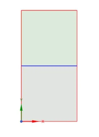
SHARE TOPOLOGY: The information between the two mediums is shared by this command

MESH:

mesh is generated under different mesh condition of different size

Mesh config	No of Nodes	No of Elements
Baseline mesh 0.5mm	3321	3200
Mesh 0.25mm	13041	12800
Mesh 0.1mm	80601	80000

FLUENT SETUP:

GENERAL:

time: transient

type: pressure based

velocity : absolute

gravity y-axis = -9.81m/s2

SETTING UP PHYSICS:

viscous: laminar

multiphase : VOF(eulearian 2 fluid) --> implicit

add material : air/user defined, water

primary phase : air/user defined

secondary phase : water

SOLUTION:

hybrid initialization is done

patching is done accordingly

RESULTS:

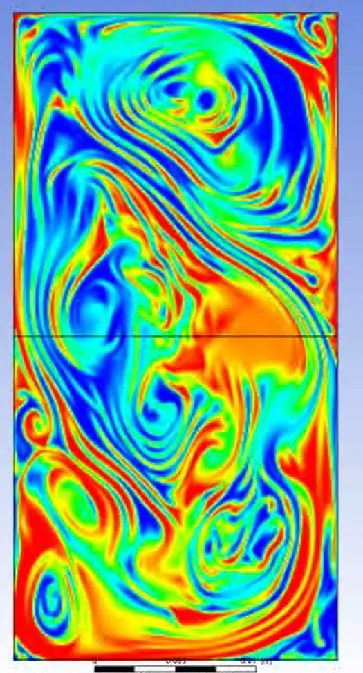
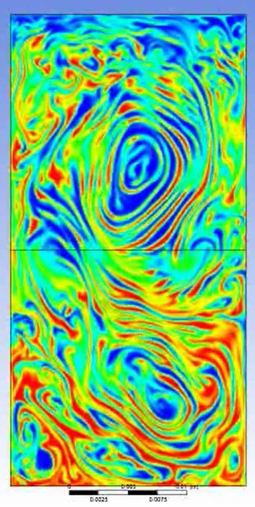
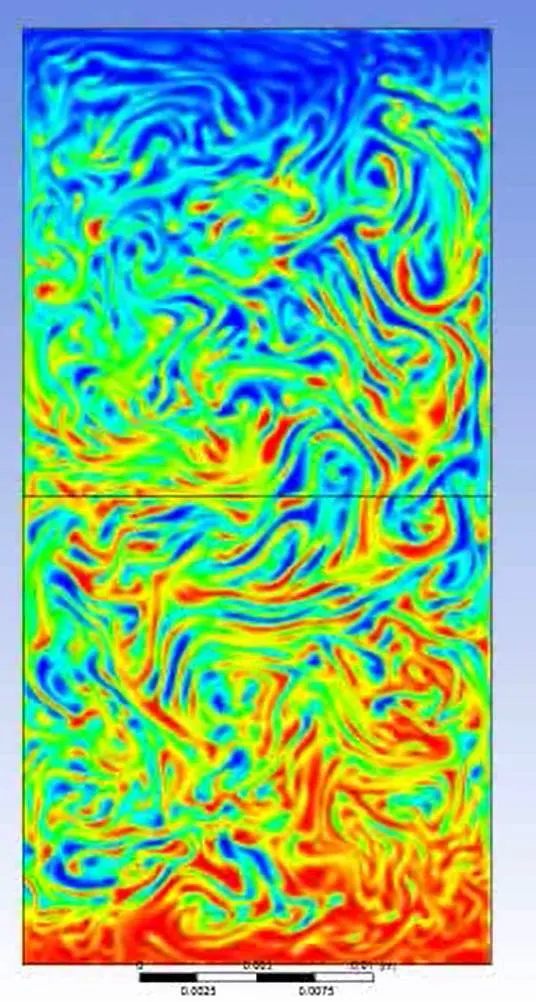
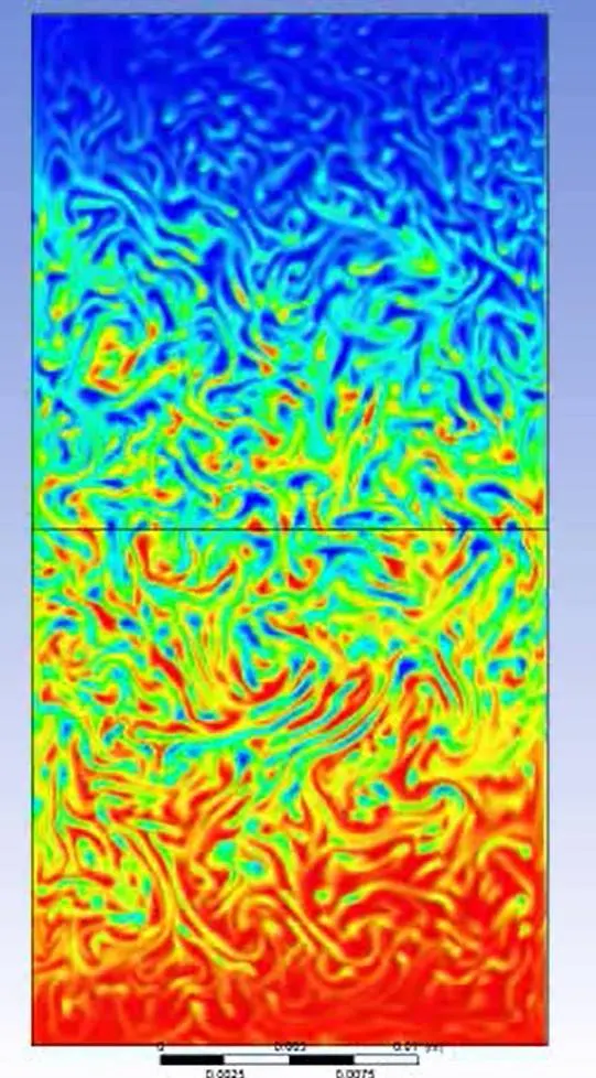
countours of phases is created.

SOLUTION: again returned to the solution and solution animations of timestep created

RUN CALCUTION:

fixed time step was set up

with time step = 0.0015(tried with different values to avoid floating point exception error)

no of time steps = 1500,2000 (depending on mesh size)

CASE-1:

1. RT_stability with baseline mesh of 0.5mm:

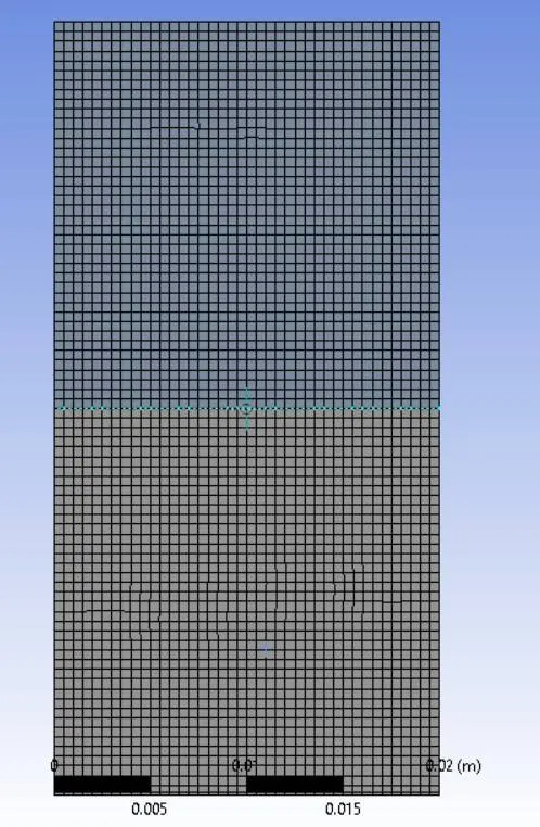
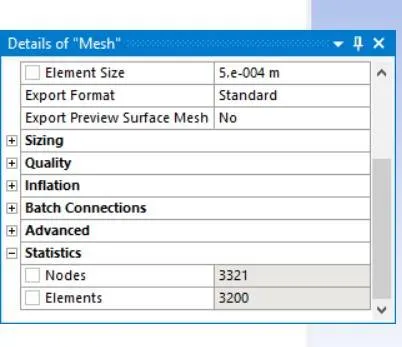
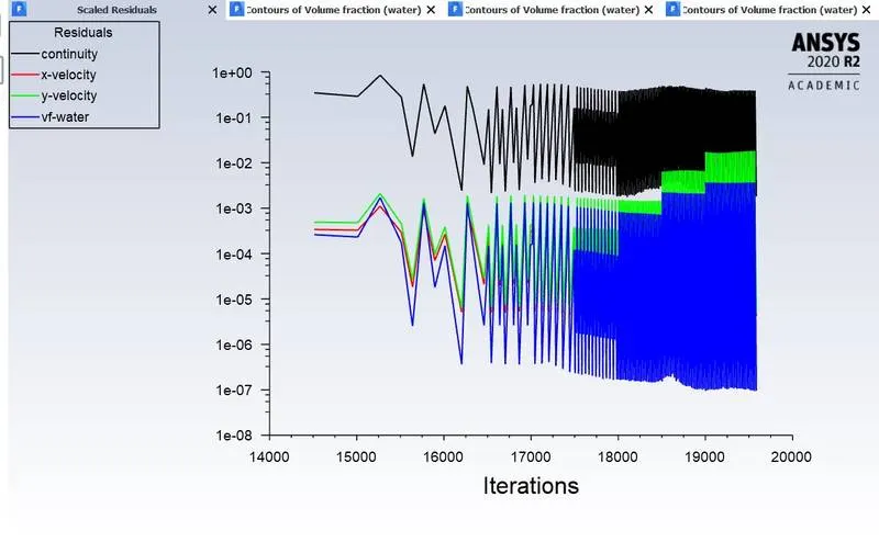
RESIDUALS: solution is converged at 18000 iteration

SOLUTION ANIMATIONS:

https://drive.google.com/file/d/1DSyK8xAJpwGaoI9LlvxoVix_Y_x6tR-v/view?usp=sharing

2. RT_stability with mesh of 0.25mm:

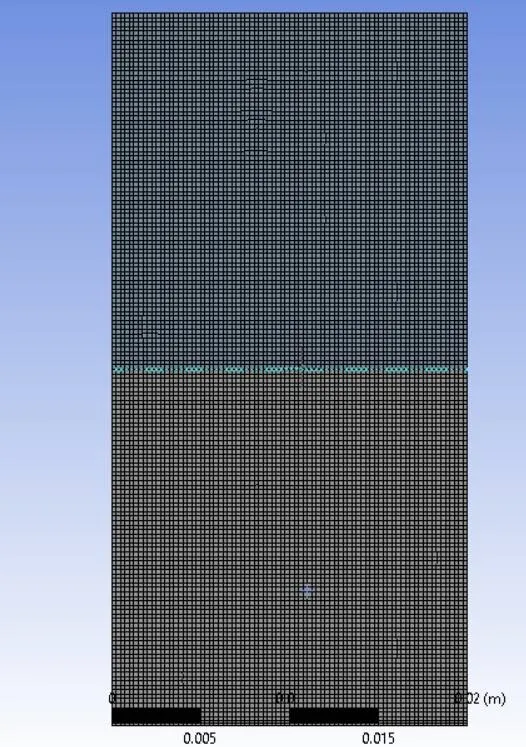
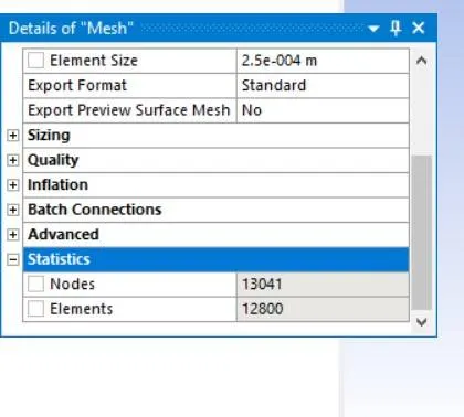
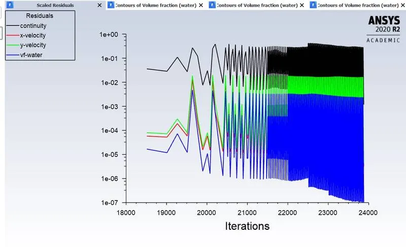
RESIDUALS: solution is converged at 22000 iterations

SOLUTION ANIMATIONS:

https://drive.google.com/file/d/19oI7-aByuewMRQ18-kwyDUHnBYyWH4o8/view?usp=sharing

3. RT_stability with mesh size of 0.1mm:

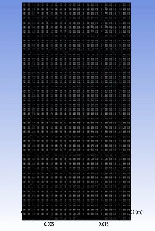
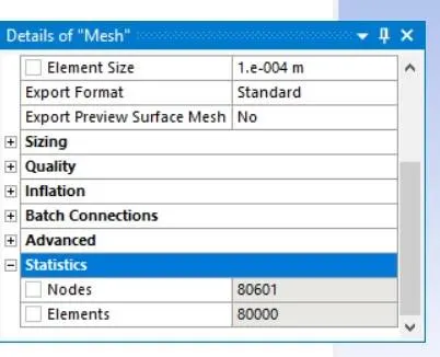
RESIDUALS: solution is converged at 29000 iterations

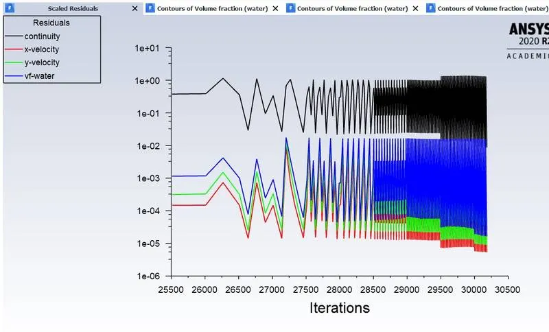
SOLUTION ANIMATIONS:

https://drive.google.com/file/d/1ZQHHyytfvsO2r5dRSK5COtNMhMp6kGIl/view?usp=sharing

CASE-2: instead of air user defined lower density material used

= density of lighter fluid = 400 kg/m3

viscosity = 0.001 Pa.s

1. RT_Stability of user defined material and water with mesh size of 0.1mm:

RESIDUALS: solution is converged at 29500 iterations

SOLUTION ANIMATIONS:

https://drive.google.com/file/d/1tQHIjR7FRo8M5oRQfeLZyBOzcAf5Kmfu/view?usp=sharing

OBSERVATIONS:

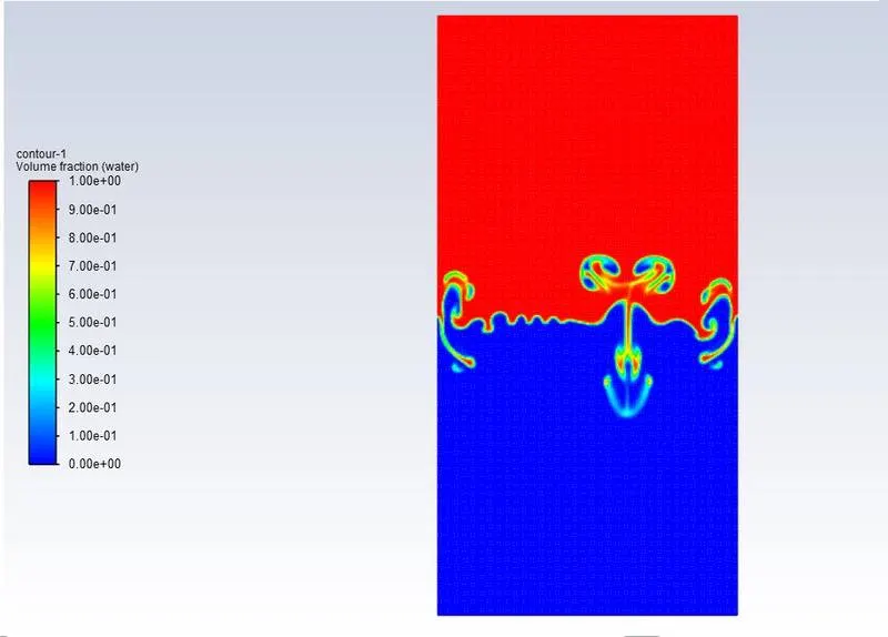
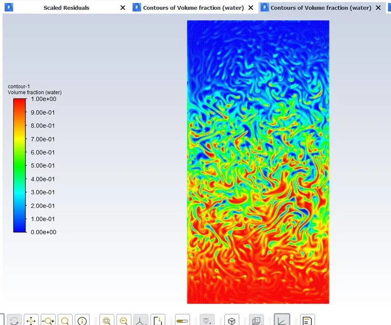
• at first the instability begins at the interfaces with small paturbations
• bubbles and spikes are generated due to density difference
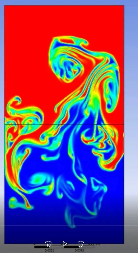
• bubbles and spikes started interacting with each other and results in turbulance mixing
• flow becomes turbulent and reynolds number increases
• after sometimes flow settles down with high density fluid at the bottom and low density fluid at the top and mixture in between and no clear inface between them is observed

WHY STEADY STATE SIMULATION IS NOT SUITABLE?

• steady state simulation is time independant approach
• based on the simulation we know that there is a very high turbulances is present and change in the flow occures in a very small time difference this is not possible to capture in steady state solver
• a stedy state solver ignores the time differentials involved in the simulation even it is able to capture the stedy state but ignores the non lineariaties in the simulation

WHAT IS ATWOOD NUMBER?

The Atwood number (A) is a dimensionless number in fluid dynamics used in the study of hydrodynamic instabilities in density stratified flows. It is a dimensionless density ratio defined as

where

= density of heavier fluid

= density of lighter fluid

FOR CASE-1:

= density of heavier fluid = 998 kg/m3

= density of lighter fluid =1.225 kg/m3

Atwood number(A)= 0.99754

FOR CASE-2 :

= density of heavier fluid = 998kg/m3

= density of lighter fluid = 400 kg/m3

Atwood number(A)= 0.42775

effect of atwood number:

With the increase in the Atwood number, the stabilization effect of initial density stratification decreases, and the instability caused by the expansion-compression effect becomes more significant. The flow structures of bubbles and spikes are quite different at medium Atwood number.

• when A is nearly equals to 1 then there a clear formation of bubbles and spikes and equilibrium achieves quicklywhen A is away from 1 difficult to differentiate bubbles and spikes due to less density difference takes more time to reach equilibrium.