Rayleigh Taylor Instability Challenge

Rayleigh Taylor instability:

The Rayleigh–Taylor instability, or RT instability (after Lord Rayleigh and G. I. Taylor), is the instability of an interface between two fluids of different densities which occurs when the lighter fluid is pushing the heavier fluid. Examples include the behavior of water suspended above oil in the gravity of earth, mushroom clouds like those from volcanic eruptions and atmospheric nuclear explosions, etc.

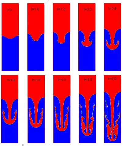
At RTI at the interface of the plane of two fluids and the heavier fluid is above the lighter fluid and under the influence of gravitational force, the shock wave is generated in the phase. Due to that, the heavier fluid starts to come down, and the lighter fluid starts to move upwards in the form of bubbles.

Some applications of RTI are in the jet engine when the fuel comes in the form of a spray.

Types of instability and some partial CFD models that have been based on Rayleigh-Taylor waves:

1) Ritchmyer-Meshkov Instability(RMI) occurs when two fluids of different density are impulsively accelerated. Normally this is by the passage of a shock wave. This instability can be considered the impulsive-acceleration limit of the Rayleigh-Taylor instability. The development of the instability begins with small amplitude perturbations which initially grow linearly with time. This is followed by a nonlinear regime with bubbles appearing in the case of a light fluid penetrating a heavy fluid, and with spikes appearing in the case of a heavy fluid penetrating a light fluid.

2) Kelvin-Helmholtz Instability(KMI) is instability at the interface between the two parallel streams with different velocities and densities, with the heavier fluid at the bottom. A common example of Kelvin-Meshikov instability is seen with the wind blowing over the water. This phenomenon is an all-encompassing occurrence of fluid flow seen time and time again in nature. From the waves of the ocean to the clouds above in the sky, the Kelvin-Helmholtz instability is responsible for some of nature's most basic structures.

3) Plateau-Rayleigh Instability(PRI) explains how a falling stream of fluid breaks up into smaller packets with the same volume but less surface area. It is related to Rayleigh-Taylor instability and it is a greater branch of fluid dynamics considered with fluid thread breakup. This fluid instability is utilized in the design of a particular type of inkjet technology whereby a jet of liquid is perturbed into a steady stream of droplets. And another example is water dripping from the tap/faucet.

Mathematical model adapted for CFD calculations:

1. Early time growth:

2. Potential flow:

3. Buoyancy-drag balance:

Rayleigh-Taylor Instability simulation:

We know that the simulation occurs in 5 stages. Geometry, Mesh, Setup, Solutions, and Results.

First in Geometry create a square with dimensions 20x20mm. Click on the pull tool and click on the surface of the body because here we are working on a 2D body. Right-click on the design and create a new component and name it air and move the surface body into the air component. Now create another component and name it water and create a new sketch and draw a square with dimensions 20x20mm and use pull tool and click on the body.

After that open workbench and click on share prep and click on yes.

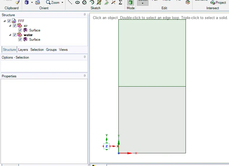
Here I am doing this project in 3 different cases with different mesh grid sizes.

Case 1(mesh grid size=0.5mm):

The mesh element size is 0.5mm.

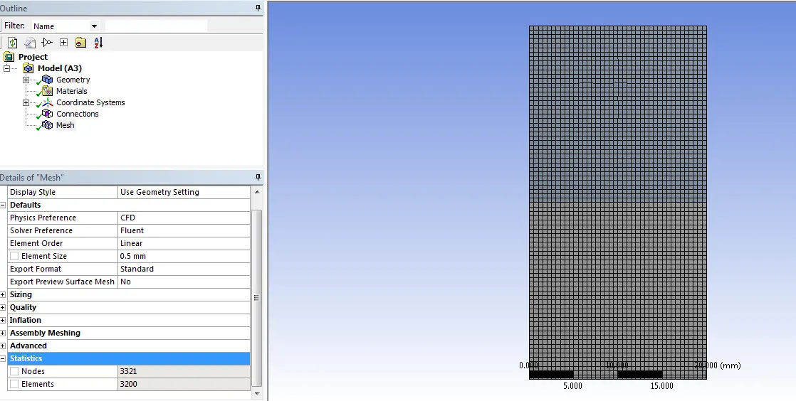
Setup:

Open setup and click on transient time (because we want to see the interface collapse as a function of time) < below that enable gravity and mention y-axis value -9.81 < open multiphase and click on the volume of fluid method and the formulation to implicit method < ok < open materials < fluent database < click on the water liquid and copy < close. In the phases < open list\show < in that change phase 1 name to air and phase material to air after that open phase 2 and rename as water and change phase material to water < close.

In solving < click on initialize and click on patch < change phase to water < click the volume fraction in variable < mention the value as 1 and select water stability < patch < and change value to 0 and select air stability < patch < close.

Go to postprocessing < open new counter < select phase counter < select water in phase < plot everywhere < save. Open animation and create animation at counter 1. Set step size = 0.005 and no. of time steps = 1500 < calculate.

Solutions:

Residuals:

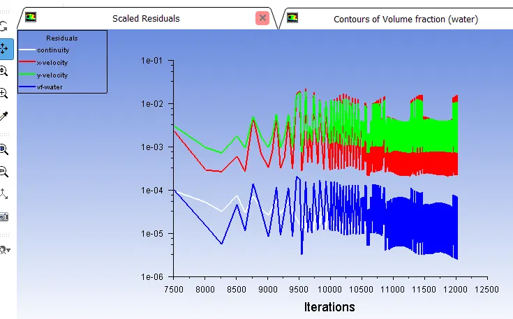
Final result:

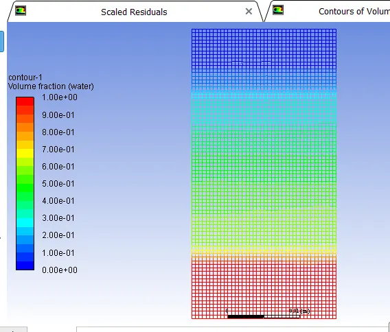
Case 2(mesh grid size = 0.3):

Mesh:

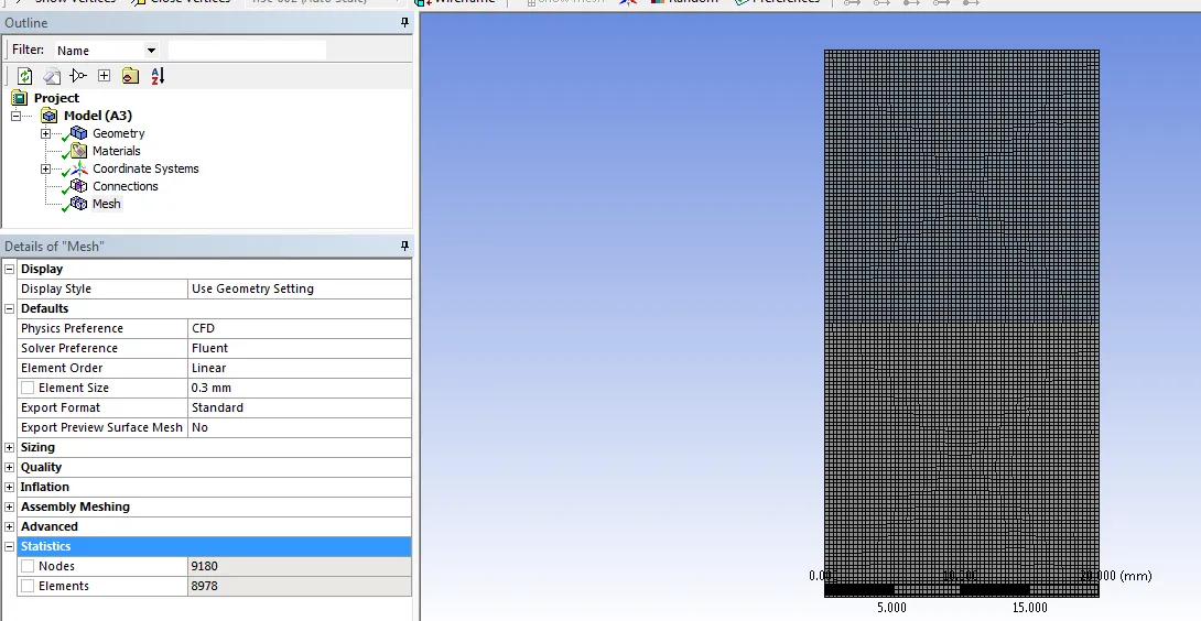
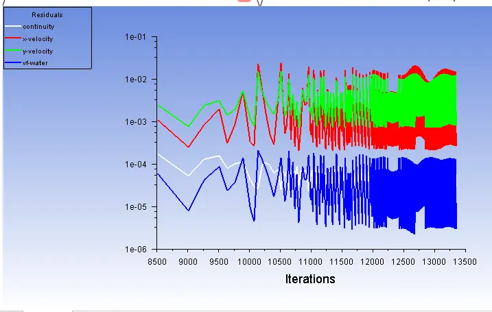
Residuals:

Velocity counter:

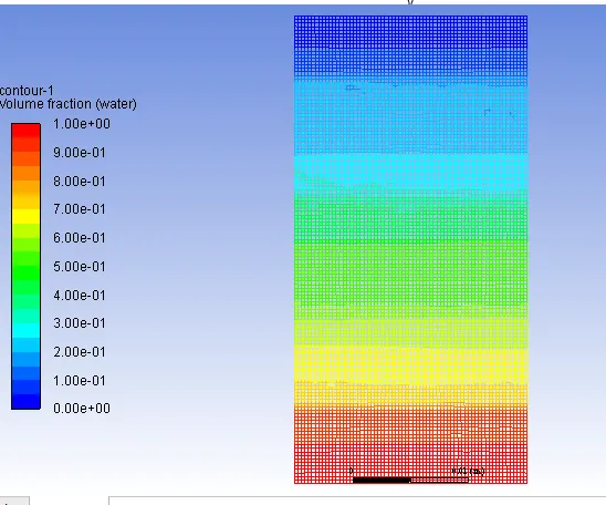
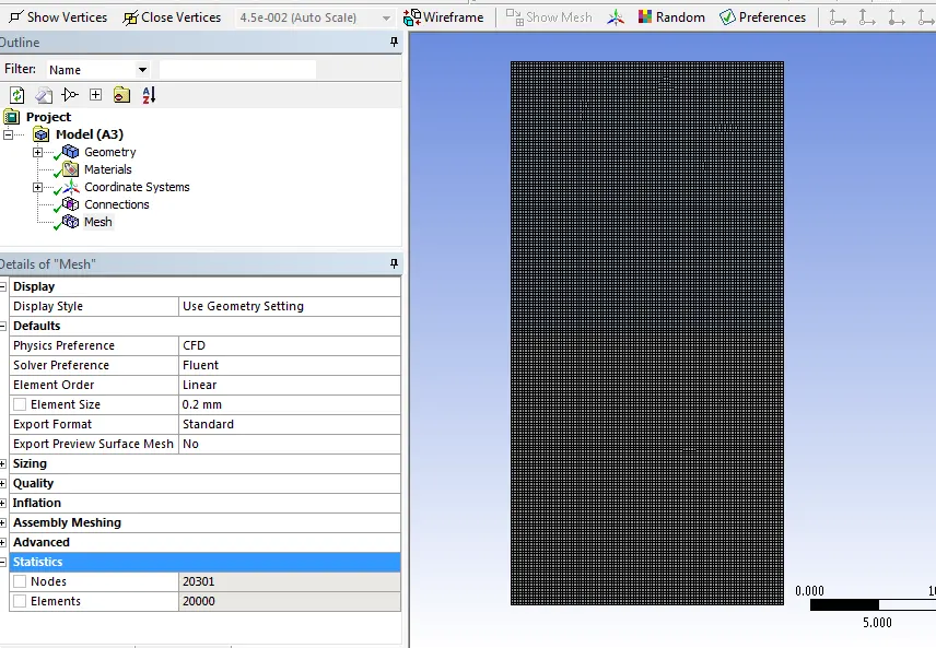
Case 3(mesh grid size = 0.2):

Here we decrease the mesh size to 0.2mm.

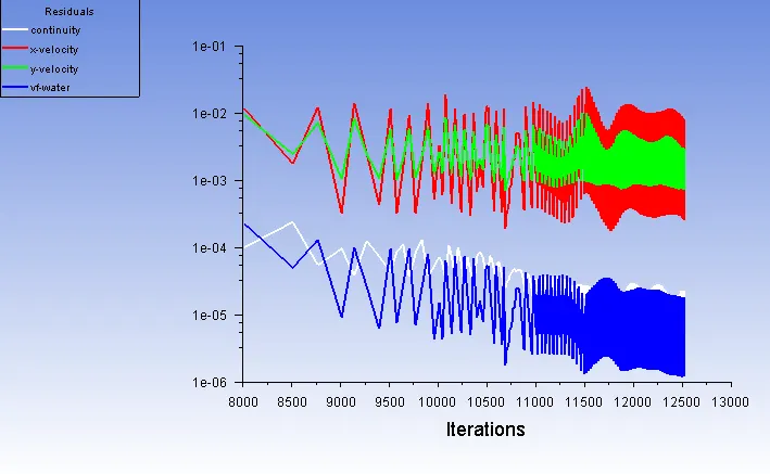
Residuals:

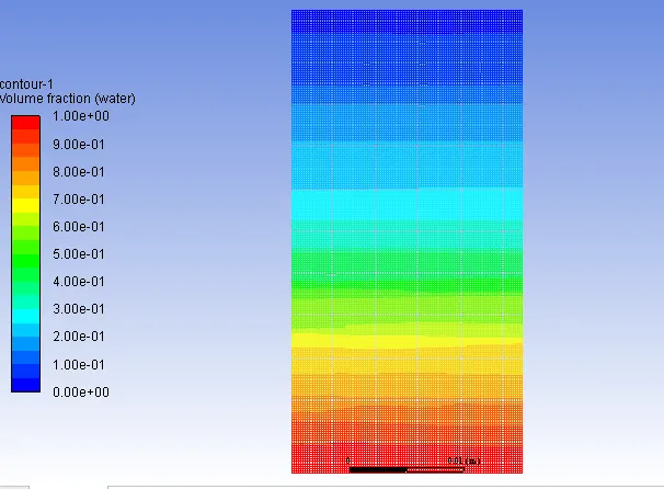
Final result:

Case 4:

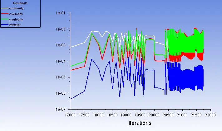
Here the mesh grid size is the same(0.2mm) but the density and viscosity of the user-defined material are changed.

Density = 400 kg/m^3 and Viscosity = 0.001kg/m-s.

Residuals:

Volume counter:

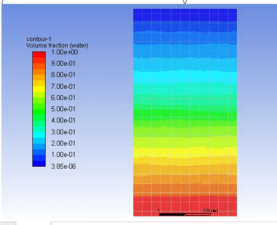
Results (Volume counter simulation):

0.5 mm:

0.3 mm:

0.2 mm:

0.2 mm with density=400kg/m^3:

Atwood number(A):

Atwood number is a dimensionless number in fluid dynamics which is used to study the hydrodynamic instabilities in density stratified flows. Atwood is an important parameter in the study of R-T Instability and in Richtmyer-Meshkov instability(RMI occurs when two fluids of different density are impulsively accelerated, normally this is by the passage of a shock wave).

It is a dimensionless density ratio defined as

A = `(rho_1-rho_2)/(rho_1+rho_2)`

`rho_1` = density of heavier fluids

`rho_2` = density of lighter fluids

In case 1 water density is 998.2 kg/m3 and air density is 1.225 kg/m3.

A = `(998.2-1.225)/(998.2+1.225)`

`A= 0.9975`

In case 4 water density is 998.2 kg/m3 and user-defined material density is 400 kg/m3.

A = `(998.2-400)/(998.2+400)`

`A= 0.4278`

Conclusion:

• By decreasing the mesh size we got a good distribution of the instability in all cases. The mixing is more fine and good.
• The Atwood number mainly depends upon the density of the materials. In case 1 the A is nearly equal to 1, thus the mixing is quite fast and takes less time to reach the steady-state, but in case 2 the A is 0.4, here the mixing is a little slow and it takes a longer time to reach steady-state.
• By this, if the Atwood number is high, then the time required to reach the steady-state is low.