Rayleigh Taylor Instability Challenge

AIM:-

To Rayleigh Taylor instability simulation for the given cases and also to give some practical CFD models based on mathematical analysis of Rayleigh Taylor waves, and also to give a definition of Atwood.

INTRODUCTION:-

Lord Rayleigh observed that when two liquids i.e. lighter and heavier fluids are mixed together where the denser fluid is top of the lighter fluid, due to the gravity the denser liquid tends to drop down and lighter liquid tends to go up. This phenomenon where two Fluids of different Densities are superposed over one another the Instability of the plane interface between the two fluids occurs this is called Rayleigh-Taylor Instability.

THEORY:

ANSYS CFD solvers are based on the finite volume method,

• Domain is discretised into a finite set of control volume.
• General conservation equations for mass, momentum, energy, species, etc. are solved on this set of control volumes.
• Partial differential equations are discretized into a system of algebraic equations.
• All algebraic equations are then solved numerically to render the solution field.

Initially, the process involves three major Categories,

Pre-Processing

• Geometry
• Mesh
• Physics
• Solver Settings

Solve

• Compute solution.

Post Processing

• Examine results.

Practical CFD models based on Rayleigh Taylor mathematical analysis:-

1. SPH method(Smoother particle hydrodynamics)

   Smoothed-particle hydrodynamics (SPH) is a computational method used for simulating the mechanics of continuum media, such as solid mechanics and fluid flows. Smoothed-particle hydrodynamics is being increasingly used to model fluid motion as well. This is due to several benefits over traditional grid-based techniques. First, SPH guarantees conservation of mass without extra computation since the particles themselves represent mass. Second, SPH computes pressure from weighted contributions of neighboring particles rather than by solving linear systems of equations. Finally, unlike grid-based techniques, which must track fluid boundaries, SPH creates a free surface for two-phase interacting fluids directly since the particles represent the denser fluid and empty space represents the lighter fluid.

2. SINGLE-FLUID MODEL

   A typical approach used for the analysis of two-phase flows is a mixture model, i.e. the individual fluid phases are assumed to behave as a flowing mixture described in terms of the mixture properties. The applied single-fluid model is a five-equation model consisting of the mass, momentum, and energy equations for a vapor/liquid mixture, and two equations describing the formation and growth of the liquid phase.

3. TWO-FLUID MODEL

   In the two-fluid model, separate sets of the governing equation for the vapor and liquid phases have been used. The interaction between the droplets and the heat exchange between the liquid phase and the solid boundary is not modeled here as well. Additionally, the velocity slip between vapor and the liquid phase is in this model taken into account.

4. Turbulence model

   Turbulence models are needed to predict the average mixing behaviour inflows that are on average one- or two-dimensional. The approach to the construction of the tile turbulence model is guided by experimental behavior. The equations governing turbulent flows can only be solved directly for simple cases of flow. For most real-life turbulent flows, CFD simulation uses turbulent models to predict the evolution of turbulence. These turbulence models are simplified constitutive equations that predict the statistical evolution of turbulent flows.

SIMULATION:-

Geometry:-

• Initially, since it is a 2 D Structure the diagram is simple.
• Using the create Rectangle tool construct a square of 20mmm, Then after constructing using the pull tool it is pulled to create a new solid.
• Then the step is repeated but keeping the base of the second square to superimpose the top of 1st Square.
• By doing so we created 2 new components.
• Share topology is selected to share the edge where the 2 squares intersects.

Meshing:-

• Initially for different cases, we are gonna use different mesh sizes and Refinement procedures.
• It is checked for proper Element Quality.

Setup:-

• After meshing the next step is to set up for proper simulation.
• We are gonna use Pressure based solver, with a Transient condition.
• Gravity is enabled and the necessary value is given in the Y-axis (i.e.-9.81) corresponding to the Geometry.
• The energy equation is disabled and the materials are added according to each individual case.
• Then a contour is created by monitoring the phase change of water by the controlled volume method.
• We are choosing a controlled volume method and selecting the implicit function.
• Finally, we are gonna use Standard Initialization to Initialize.
• Then we are going to patch the different phases by selecting the water and control volume method and number 1 for water fluid.
• Then 0 is given to other material say air or user-defined material.

Case-1:-

• It is a baseline Simulation consisting of a mesh size of 0.5mm.
• We are going to use Water as High-Density Fluid and air as Low-density Fluid.

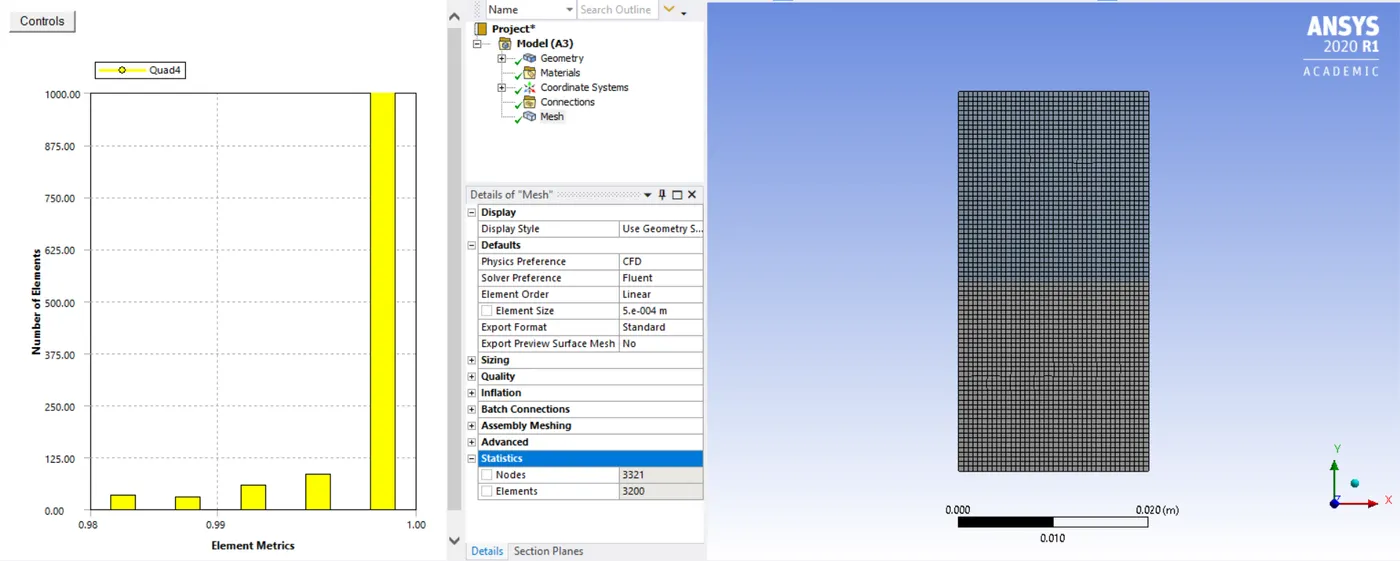
Baseline mesh of element size 0.5mm

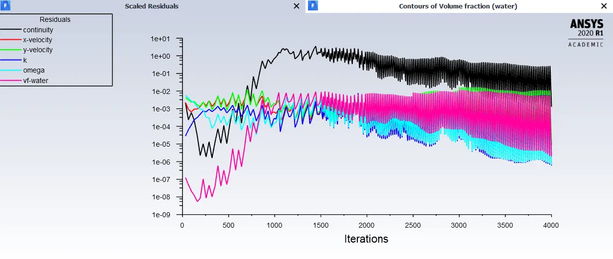
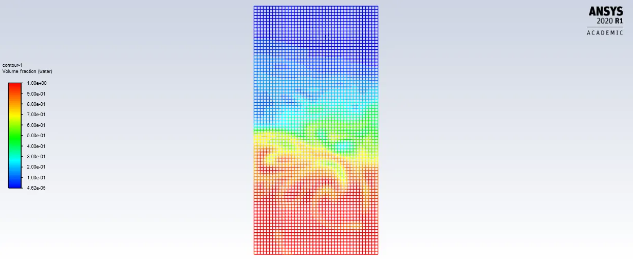
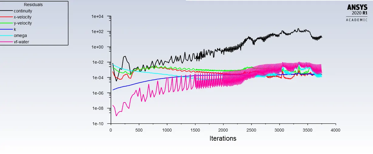
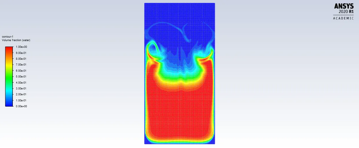
Scaled Residuals Final Image after Simulation

Baseline simulation

CASE-2:-

• It is a Refined simulation having a Mesh element size of 0.2mm.
• It also uses the same materials for Light and Denser fluids, i.e. Air and Water.

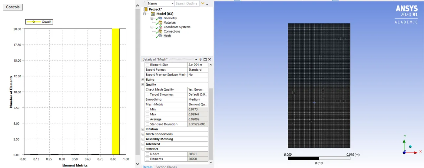
Refined Mesh and Corresponding Element Quality

Scaled Residuals Final Image of Refined Simulation

Refined Simulation

CASE-3:-

• It is a Refined simulation having a Mesh element size of 0.2mm.
• We are going to use Water as High-Density Fluid and User-defined material as Low-density Fluid.
• User-defined material has 400Kg/m e3 of Density and 0.001 Kg/m e-1.

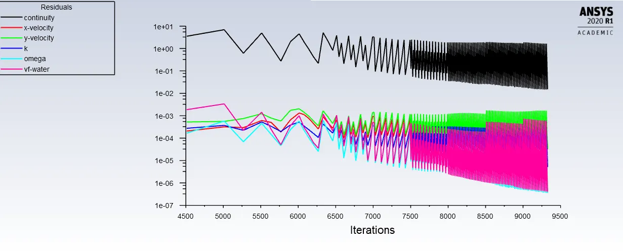
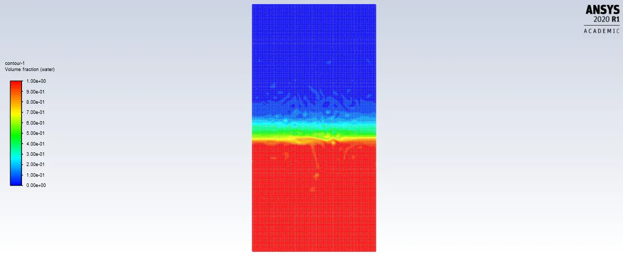
Scaled Residuals Final Image of Refined Simulation using user-defined material

User-defined simulation of Rayleigh Taylor Instability

OBSERVATION AND CONCLUSION:-

In the above cases, the simulation starts with the state of hydrostatic equilibrium, and the Rayleigh Taylor instability is observed at the interference when a lower density fluid pushes a higher density fluid due to which formation of shock waves at the interface takes place. The formation of air bubbles starts taking place, which compresses the heavy fluid around it, due to which shock waves of multidimensional fashion generates and it gets stronger as it moves upward. It is observed that the more we refine the mesh, the more the simulation results get smoother about the irregularities that take place at the interface of the two fluids. As higher density fluid replaces lower density fluid, the formation of air bubbles and vortex takes place, which travels towards the upward region with time. In case-2, we can see the more detailed results about the formation of waves and the formation of some air bubbles that get trapped at the lower region during the initial stage and then they travel towards the upper region, generating shock waves. At the end of the simulation, it is to be observed that the two phases get separated from each other though, we can see some diffusivity between them which is a volume fraction of air and water.

Why a steady-state approach might not be suitable for this Simulation:-

The difference between the steady and transient is that you can't see the small-time variation of instability. The steady-state simulation is performed if we are concerned more about the final state results or the equilibrium state. In RT-Instability CFD models, we are more concerned to learn about the transition of the irregularities that starts developing when we pour high dense fluid upon low dense fluid under gravity effect so, by using a transient solver along with the refined mesh of the model, we can compute the smooth transition of irregularities that takes place at the interface of the fluids. The final state results for both the steady-state and transient state will be the same.In this problem we are observing the instabilities when it is occurring so we are not concerned about the final answer because a steady-state is more into capturing the final results but by transient, we can see the behavior of the solution and every instant such that capturing bubbles, vortex and Shockwaves. So this is the reason why transient is more suitable than the steady-state model.

Atwood Number:-

The Atwood number (A) is a dimensionless number in fluid dynamics used in the study of hydrodynamic instabilities in density stratified flows. It is a dimensionless density ratio defined as-

A = `p1-p2`/ p1+p2.

where

p_l= density of heavier fluid

p2 = density of lighter fluid

Atwood number for above cases-

A=(1000-1.25)/(1000+1.25)=0.9975

For Atwood number close to 0, RT instability flows take the form of symmetric "fingers" of fluid;

For Atwood number close to 1, the much lighter fluid "below" the heavier fluid takes the form of larger bubble-like plumes.