Rayleigh Taylor Instability Challenge

RAYLEIGH TAYLOR INSTABILITY

1. PROBLEM STATEMENT:

• Some practical CFD models that have been based on the mathematical analysis of Rayleigh Taylor waves and explain how these mathematical models have been adapted for CFD calculations.
• Rayleigh Taylor instability simulation for 2 different mesh sizes with the base mesh being 0.5 mm. compare the results by showing the animations. Observation for the differences in the animation and explain the effect of mesh size on simulation.
• Explanation for why a steady-state approach might not be suitable for these types of simulation.
• Air and Water should be chosen for this simulation. Simulation comparison with water and user-defined material (density = 400 kg/m³, viscosity = 0.001 kg/m-s) for refined mesh.
• Define the Atwood Number. Find out the Atwood number for both the cases and explain how the variation in Atwood number in the above two cases affects the behaviour of the instability.

2. PRACTICAL EXAMPLES BASED ON RAYLEIGH TALOR INSTABILITY:

RT instability or RTI is the instability commonly seen during the phase interaction and mixing of two different density fluids. The disturbances can be stated by the visualisation of the lighter fluid pushing the heavier fluid. Various common examples can be stated as:

• Water suspended over the oil column with the effect of gravity: The difference in the density of water and oil under the effect of gravity leads to the instability arising from the phase interaction point to the point where the heavier fluid whole settles downwards after definite time and obviously the lighter one at the top. The process and the instability which can be seen during this phase interaction till the stability in the phase is achieved is what we call Rayleigh Taylor instability.
• Mushroom like clouds that can be seen in a volcanic eruptions or in any nuclear explosion: These can be seen with a clear visualisation that the lighter domain region is what takes the shape of the mushroom during the instability or phase interaction. In other examples stated above heavier domain forms the shape of a spikes at the initial disturbances and lighter domains forms the shape of the bubbles or mushroom kind.
• Supernova explosions: Where the expanded core gases are accelerated into the heavier medium of shell gases. Instability in the plasma fusion reactors are also one of the examples.

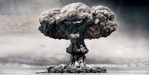
Fig: Pictorial example of RT instability

3. ADOPTION OF MATHEMATICAL MODELS FOR RT INSTABILITY CFD CALCULATIOS:

The mathematical model involves basically two methods named as:

• Diffused interface method and
• Boussinesq’s approximation model

The governing differential equation involved in it is the Navier-stokes equation in which the momentum equation requires the Boussinesq’s approximation. The differential equations incorporated in it are as follows where β is the compressibility factor for the artificial compressibility method

∂p/∂τ+β (∂u/∂x+∂v/∂y) =0 (i)

∂u/∂τ+∂u/∂t+∂ (u²+p)/∂x+∂uv/∂y−μ (∂²u/∂x²+∂²u/∂y²)

= −λ (∂ϕ/∂x) (∂²ϕ/∂x²+∂²ϕ/∂y²) (ii)

(∂v/∂τ) + (∂v/∂t) + ∂ (v²+p) ∂y + ∂uv/∂x – μ (∂²v/∂x²+∂²v/∂y²) =

−λ (∂ϕ/∂y).ƿ (∂²ϕ/∂x²+∂²ϕ/∂y²) – g (ρ1−ρ2) ((1+ϕ)/2) (iii)

The diffused interface method incorporates into it the following function considering that the domain of fluid phase function as:

ϕ(x, t) for x ∈ Ω for

F (ϕ, ∇ϕ) =∫Ω (1/2|∇ϕ|²+1/4η² (ϕ²−1)²) dx

The Boussinesq’s approximation model incorporates the following equation for the momentum equation in the Navier-stokes equation for the small density variation:

ƿ _o [u_t + (u.∇) u] = −∇p̃ + ∇.σ + b (ϕ)

The usual meaning of the notations used are to be followed and the above used and then the equation is being discretised to get the results for the 2D simulation of the Rayleigh Taylor instability

The equation above stated almost all involves the variation w.r.t time both pseud and physical

The pseudo time step represented as τ and the physical time as t is being used in the governing differential equations and both Neumann and periodic boundary conditions has to be applied for getting the calculations.

4. GEOMETRY:

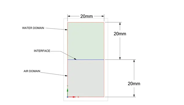
Fig: geometry showing the different fluid domain

5. SIMULATION COMPARISION OF DIFFERENT GIVEN CASES:

5.1 BASE LINE MESH: 0.005 m element size mesh

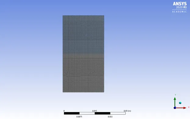
Fig: mesh for base line simulation

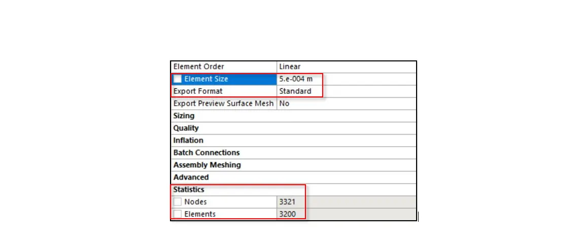
Fig: mesh details

5.1.2 MODELLING METHODS AND PHYSICS:

This simulation comes under the MULTIPHASE modelling method in which the two different fluids used are taken as water and air where air being the lighter is initially kept lower and water the heavier is kept above so as to obtain the instability when the perturbation starts

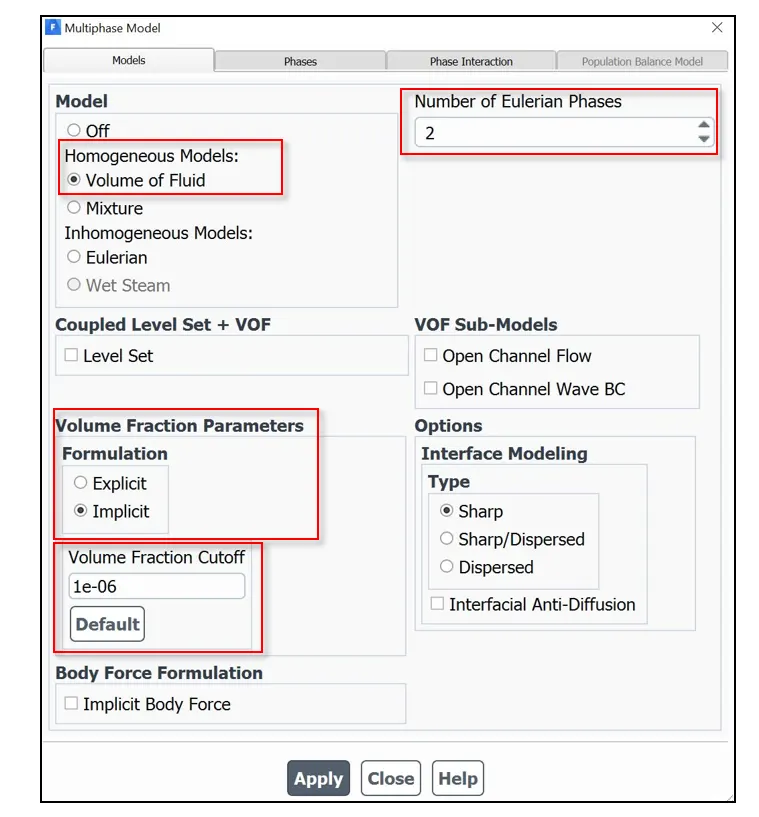
Fig: Multiphase model details

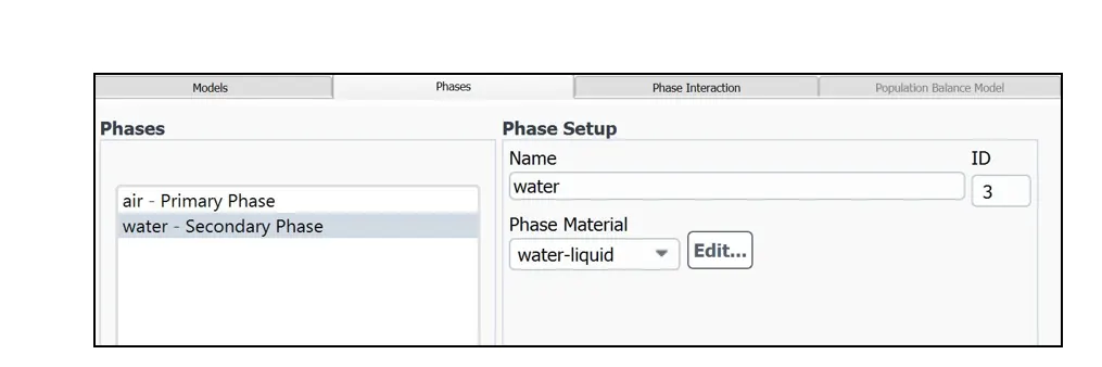
Fig: Defined phases

The viscosity section of ANSYS Fluent was simply chosen as the laminar flow type & the predefined material properties of the fluids selected are left as it is.

No boundary conditions are separately provided and are considered only in the multiphase model itself. Also standard type initialization is being done before the calculation to be performed and each case simulation performed is for total of 1 second time.

The time steps size and the total number of time steps for the calculations has to be varied continuously so as to keep the time step size in order with the changing mesh size and its calculations performed to avoid any floating point error.

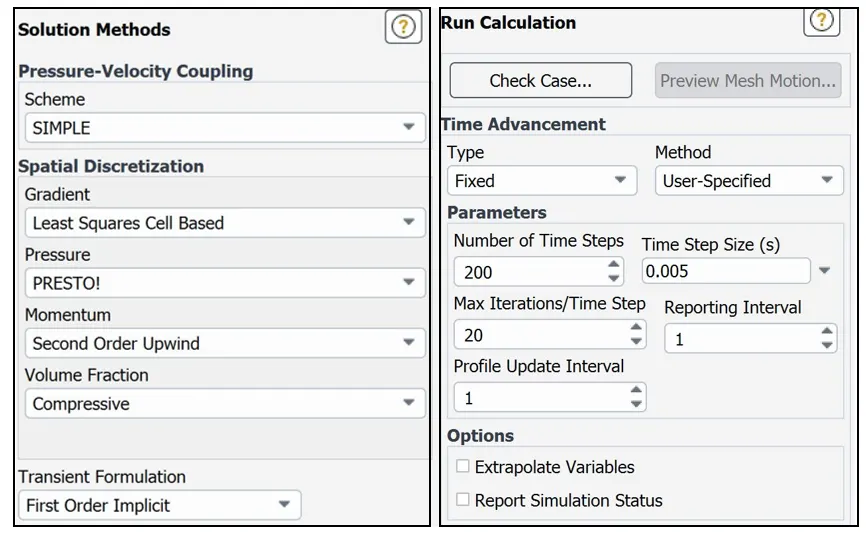
Fig: method involved and calculation parameters

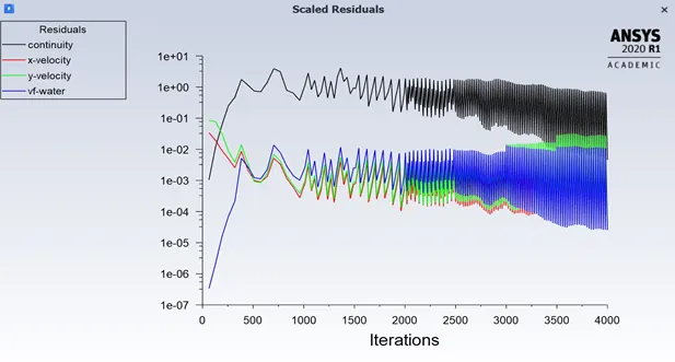
Fig: transient residual plot for simulation for 0.005 m mesh

5.1.3 RESULTS FOR BASELINE SIMULATION AT DFFERENT TIME:

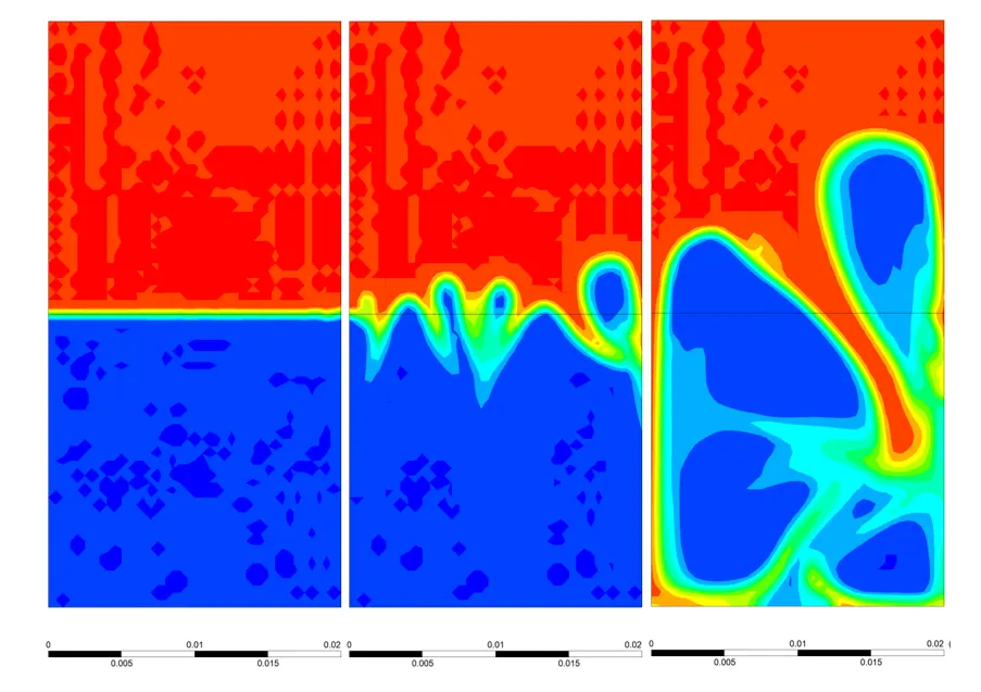
0 sec 0.1 sec 0.2 sec

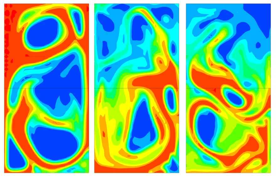
0.3 sec 0.5 sec 0.6 sec

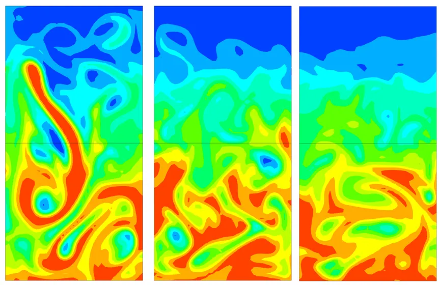
0.7 sec 0.9 sec 1 sec

ANIMATION FOR THE ABOVE CASE:

https://drive.google.com/file/d/1rowqp47h6utnt-8jTNHlC-BkJkZMxX8u/view?usp=sharing

5.2 CASE (ii) mesh size 0.00025 m

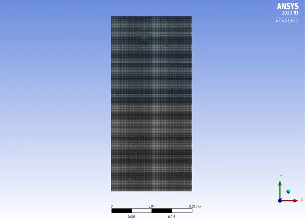
Fig: Mesh for 0.00025 m case

The total time for which the simulation is being run for here is 1 sec only but as the mesh size in this case is a bit smaller than the previous case so the time step size should be a bit smaller as we can keep it same as we keep on reducing the mesh element size up to certain limit. Although after running for this case with the same time step it was fine as per the requirement for the calculation of software thus we kept it same for this case as the previous case.

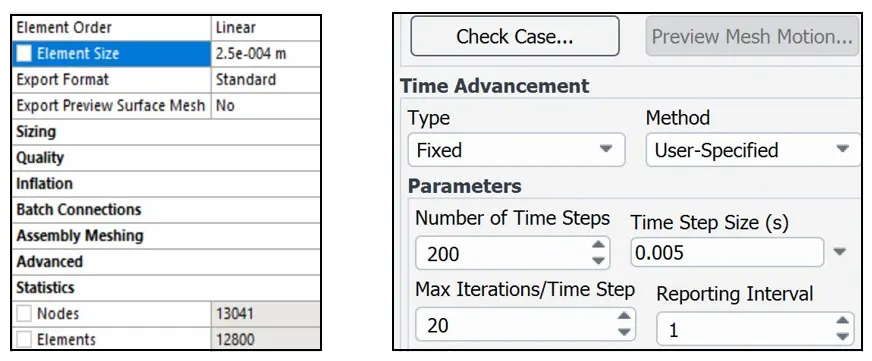
Fig: Mesh details and calculation details

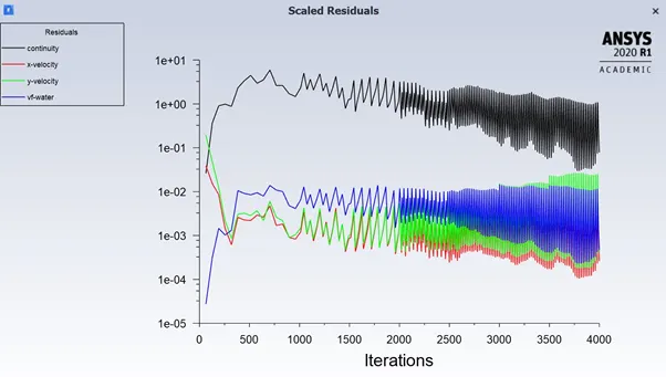
Fig: Residuals

5.2.1 RESULTS FOR CASE (ii)

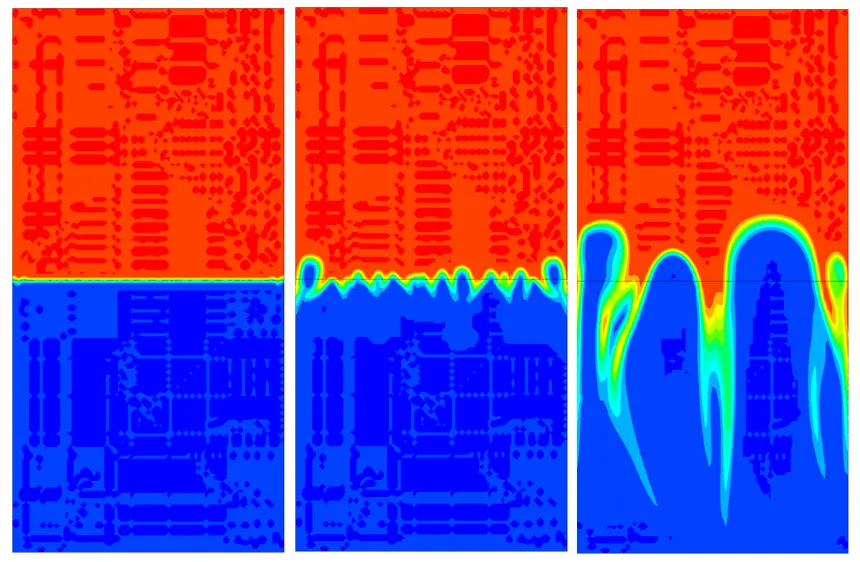
0.025 sec 0.05 sec 0.1 sec

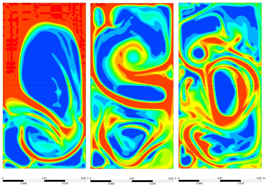
0.3 sec 0.4 sec 0.5 sec

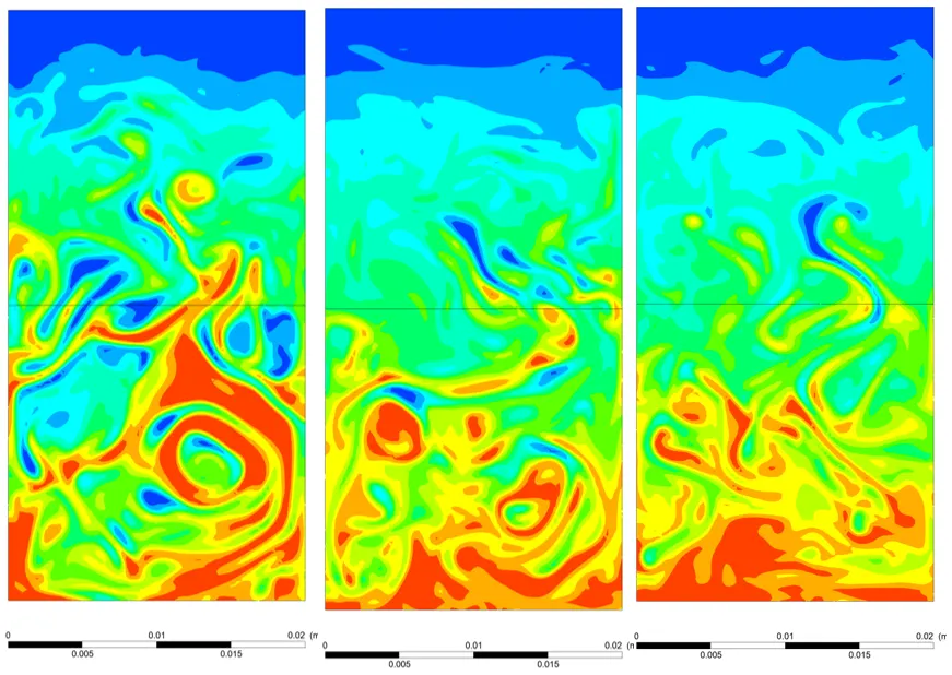
0.7 sec 0.9 sec 1 sec

ANIMATION FOR THE ABOVE MEDIA:

https://drive.google.com/file/d/1yyCDk-5SOrlFXTNODtNHWt97Rc8iZdVK/view?usp=sharing

5.3 CASE (iii) mesh size 0.0001 m

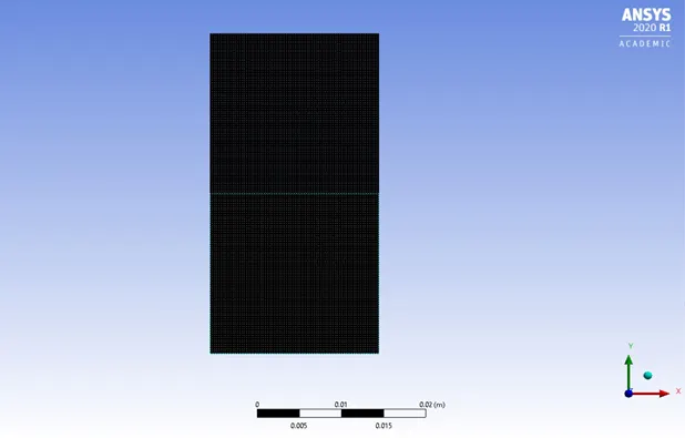
Fig: Mesh for 0.0001 m

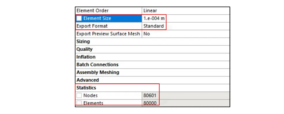
Fig: mesh details

The calculation for the system wasn’t feasible this time for the same time step size given that the mesh size has been reduced like 5 times of the mesh element of baseline meshing thus the time step size was here reduced to 0.001 and the total steps was for 1000 steps thus making the total time for simulation to be 1 second only like all other cases for a better comparison among them.

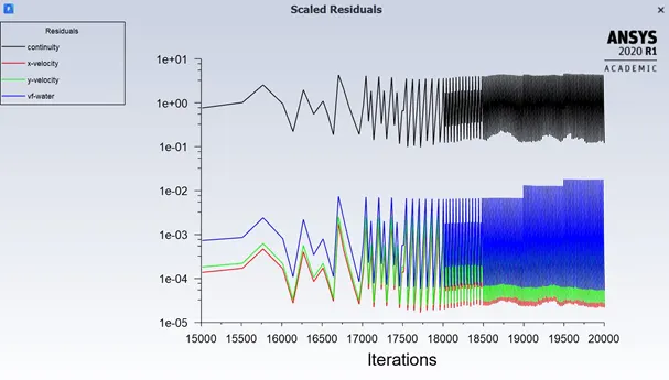
Fig: Residuals

5.3.1 RESULTS FOR CASE (iii):

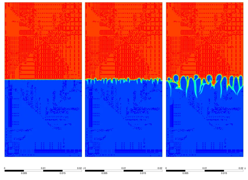
0.06 sec 0.08 sec 0.1 sec

• In this meshing case the 1^st instability can be clearly seen at very initial time 0.06 sec itself which couldn’t be seen clearly as in the case of coarser mesh case.
• A proper mushroom kind of bubbles can be clearly seen in the most refined case here. The denser fluid here shown in the bottom domain initially here shows to be gong upwards as its place is replaced by the heavier fluid which comes down in form of spikes in the effect of gravity. The refined mesh clearly shows that it gives a better detailed view of instability than previous cases of coarser mesh.

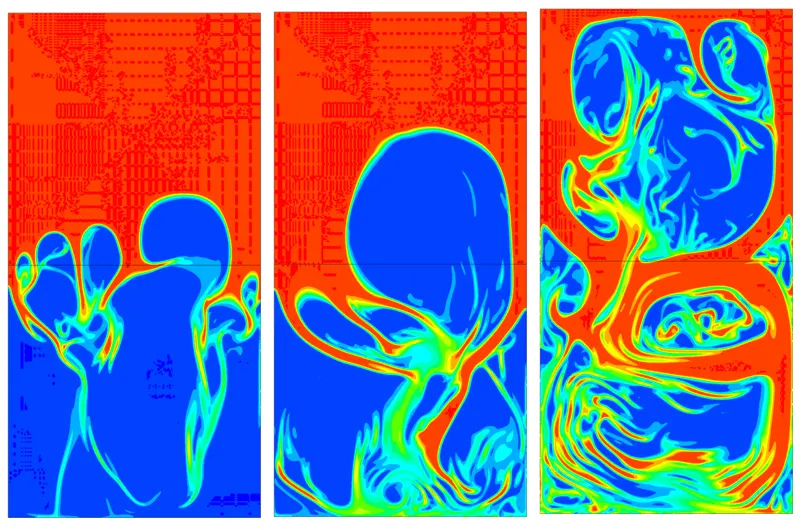
0.15 sec 0.2 sec 0.3 sec

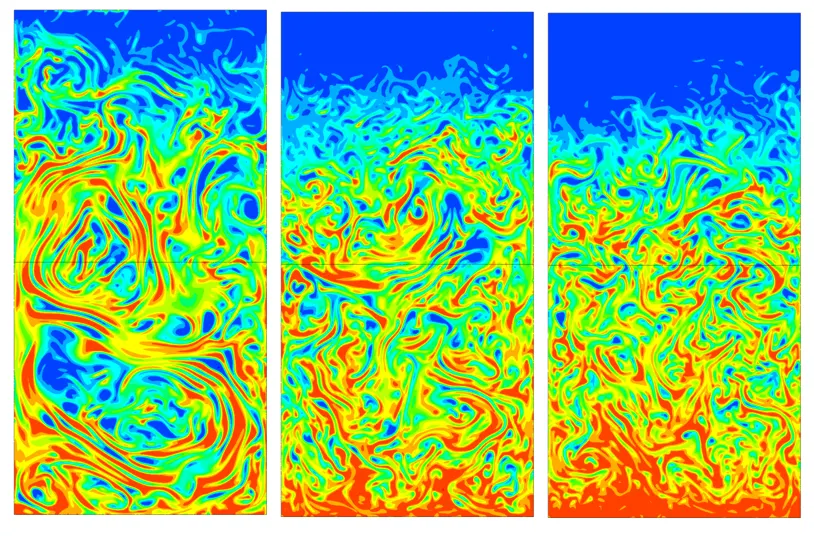
0.5 sec 0.8 sec 1 sec

ANIMATION:

https://drive.google.com/file/d/1sbTv_y6MIDgFlLLo_8KtIa7-9PU4JMAf/view?usp=sharing

5.4 CASE (IV) USER DEFINED MATERIAL CASE FOR REFINED MESH:

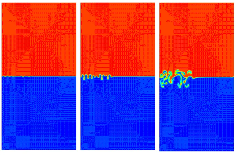
0.17 sec 0.2 sec 0.25 sec

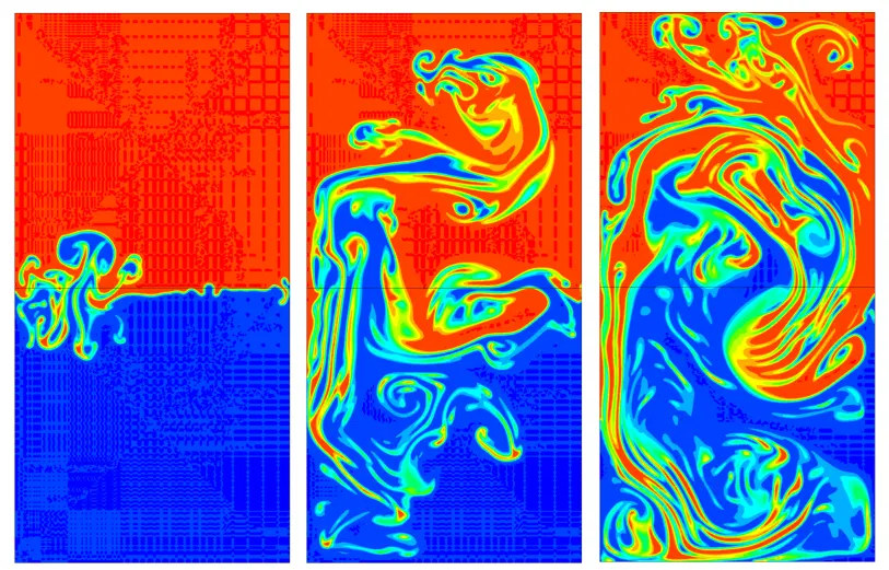
0.3 sec 0.5 sec 0.6 sec

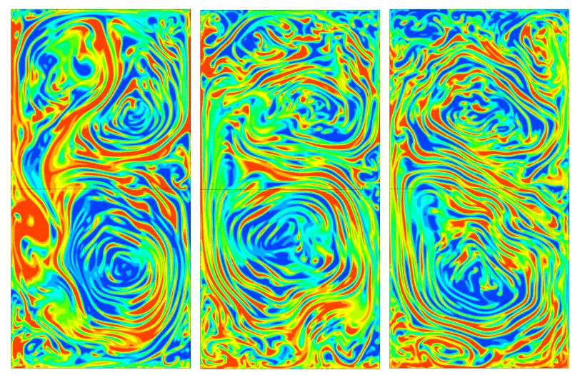
0.8 sec 0.9 sec 1 sec

ANIMATION LINK:

https://drive.google.com/file/d/17bYA9hkeodx0syUEDdf7D9xaltYUFPQ3/view?usp=sharing

CONCLUSION FROM THE WATER-AIR CASE & USER DEFINED CASE:

The below comparison shows that the water –air interface when comes into interaction with each other shows the sudden spikes formation in it at very initial stage itself and the perturbation starts too quickly which isn’t seen in the case of the user defined fluid which has here greater viscosity and density as compared to the air in the previous medium thus at every equal time step also shows delay in instability and lastly the stabilization of the lighter and heavier domain w.r.t time.

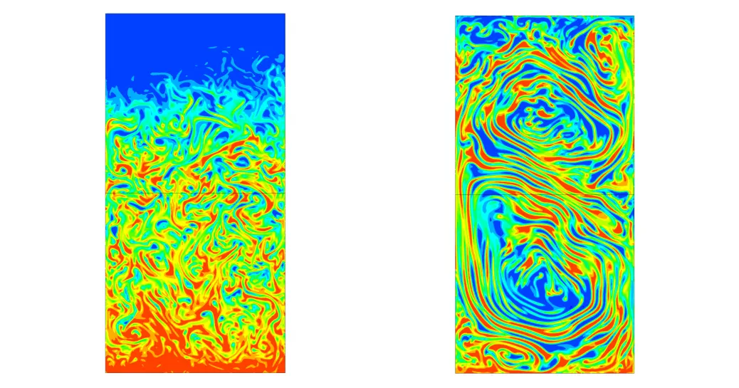
0.0001 m mesh water-air domain at 1 sec User defined case with water at top at 1 sec

6. ATWOOD NUMBER & ITS EFFECT ON THE INSTABILITY:

Usually to be seen in hydrodynamic instabilities the dimensionless number Atwood number is used in fluid dynamics where density stratified flows are being studied.

Mathematically we defined this dimensionless number as:

A= (ƿ1-ƿ2) / (ƿ1+ƿ2)

A for water-air domain = 0.9975

A for the user defined domain = 0.4278

Where clearly the ƿ1 is the heavier fluid and the ƿ2 is the lighter fluid thus making the value of Atwood number always less than 1. This Atwood number value as per depending upon the fluid used regulates the instability depending upon certain formulations

Thus now as per the significance of it on the stability is concerned we can explain this by the initial perturbation formula which occurs initially when the heavier fluid is above the lighter one and the perturbation which starts occurring have an exponential nature defined by the equation below:

exp (γ t)

With γ =√Agɑ

Where the γ signifies the temporal growth rate i.e. time dependent growth rate and the ɑ denotes the spatial wave number i.e. space dependent and as usual A denotes the Atwood number

Thus the above mathematical nature of the initial perturbation and its continuity in exponential nature which incorporates the time dependent constants like γ will give better GUI simulations and will give the similar results to that of theoretical simulations only if run on the basis of unsteady state simulations.

The time evolution of the free interface is being stated here below where B is the amplitude of the initial perturbation and the R denotes the real part.

η= R {B exp ((√Agɑ)*t) exp (iɑx)}