Exhaust Port Challenge

EXHAUST PORT COJUGATE HEAT TRANSFER SIMULATION

1. PROBLEM STATEMENT:

• Brief description of where and why CHT analysis is used
• Maintain the Y+ value according to the turbulence model and justify the results
• Wall and surface heat transfer coefficient on the internal solid surface and the velocity and temperature contours in the appropriate areas
• Verification of the HTC from the simulations and factors on which its accuracy depends

2. INTRODUCTION:

Heat transfer problems can be considered into the various aspects like conjugate, coupled or adjoint simulation. These terms corresponds to the problems consisting of two or more subdomains based on distinct differential equations depending upon the method used. The heat transfer between a body and a fluid flowing past it, is a conjugate type of problem, because the heat transfer inside the body is governed by the elliptical Laplace equation or by the parabolic differential equation, whereas the heat transfer inside the fluid is governed by the elliptical Navier-Stokes equation or a parabolic boundary layer equation. The solution of such problem gives the temperature and heat flux distributions on the interface. Thus the CHT is the situation where a solid and fluid interacts with each other and we need to know the thermal exchange at the interface or within the solids and fluids. One of the example of it can be hot or cold air moving past a solid body and resulting to the change in its temperature.

3. AIM:

The prior aim of the analysis is to verify for a particular turbulence model for its Y+ range if it lies in the correct zone. We have to also determine surface HTC in an appropriate region so that we can know how the value of HTC varies in the internal solid surface and in the inflation layers. The support for all the verifications will be given with the help of temperature and velocity plots at different regions.

4. THEORY BEHIND THE APPLICATIONS OF CHT & TURBULANCE MODELS:

CHT analysis can be performed to improve the cooling of the water jacket and improve the engine life among many other applications. Critical cooling applications most of the time depends on multiple thermal protection techniques, like internal, external film cooling, etc. which are efficiently used in our analysis to cool components and limit the use of coolant.

The below listed models are generally used to turbulence modelling because of the need of additional equations for making the problem closed.

Spalart-allmaras model is 1 equation model, which are developed and used extensively for aerospace industry application. On the other hand k- omega and k- epsilon are two equation models. These are semi-analytic models by the way. k- Epsilon model predicts far from the boundaries (wall) & k- omega model predicts well near wall. Even though it depends on Y+. We also have SST model which is a combination of these. Selection of model depends on the specific problem, no turbulence model is suited for the every case. Fine tuning is required. SST model used good mesh at boundary and with wall treated usually works in most cases, but again it is problem specific and we need to do the analysis of different kind and with different physics for all the cases which suits it. In this particular steady state simulation we are going to analyse the simulation through an exhaust port with total four inlets coming from the 4 cylinder engine and then resulting into a single port of exhaust outlet. The velocity and temperature variations among the different solid sections and inside the intricate shapes of the exhaust port needs to be shown to have better understanding of the flow characteristics with respect to its fluid section and the boundary layers.

5. GEOMETRY, CAD MODEL & MESHING:

Below CAD shows the geometry with 4 inlet ports and one outlet port of the solid model which will be the part of the conjugate heat transfer. No duplicate edges were found before doing the meshing part and it should be checked upon.

Fig: Exhaust port CAD model outlet dimensions

Fig: Exhaust port CAD model inlet and other view dimensions

5.1 FLUID VOLUME EXTRACTION:

The below region of volume shows the fluid region in which the air as a fluid at temperature of 700 K flows through and channel and goes out through the outlet port.

Fig: Fluid volume extracted

5.2 NAMED SELECTION PARAMETERS:

The named parameters for selected for inlet and outlet faces are being shown in the below diagrams

Fig: Inlet, outlet, inflation layers and surface wall parameters

5.3 MESHING:

Fig: Solid-Fluid Meshing

INFLATION LAYERS:

Before creating below inflation layer greater number inflation layers were given at 1^st for the analysis to check if it gives the results within the preferred limits. Total 6 layers were selected at 1st as inflation layers with the total thickness of 8mm considered for the max inflation thickness and growth factor of 1.2. this case Y+ value would be set up for the K-epsilon turbulence model in which the Y+ was range from >30 value and many values ranged outside the buffer zone thus K-omega model was selected and for which the aim is to get the maximum or all Y+ value of a region to be within 0-5 of range thus the inflation layers are reduced to total 3 layers & maximum inflation layers thickness was kept 0.5mm.

Fig: Inflation layers

5.3.1 MESH DATA:

The minimum mesh metric data here is seen to be around 13% which is appreciable and we can go with the further calculations:

Fig: Mesh element size

5.4 MESHING DETAILS FOR MINIMUM MESH METRIC DATA:

This particular case defines the condition for the lesser Y+ value in a range of 0 to 5 for k-Omega turbulence case and can be later verified with the theoretical calculations where the value of Y+ can be determined using the parameters such as kinematic viscosity, value of Y and wall friction velocity.

Fig: Mesh metrics for thinner inflation layers case

Fig: Inflation layers data

Fig: Minimum mesh metric value

6. SOLVER, DISCRETIZATION, PHYSICS AND MODEL:

The Solver here is Pressure-Based with absolute velocity formulation and steady time. The model used here is the turbulence model of K omega of SST type. The preferred reason for the selection of k-omega SST model here is because k omega is much more preferred in the case of near wall conditions and we want the analysis much precise near the wall so as to get the more accurate HTC and other contours analysis like near wall temperature and velocity near walls at certain regions of inflations.

Solution method used here are:

• Coupled Pressure-Velocity coupling
• 2^nd order Pressure
• 2^nd order Momentum upwind
• 2^nd order KE upwind
• 1^st order specific dissipation rate
• 2^nd order upwind Energy

7. FLUID & SOLID MATERIAL USED AND IT’S PROPERTIES:

TABLE I:

Material	Density(kg/m^3)	Specific heat(J/kg-K)	Thermal Conductivity(W/m-K)	Viscosity(kg/m-s)
Fluid (AIR)	1.225	1006.43	0.0242	1.7894e-05
Solid (Aluminium)	2719	871	202.4	---

7.1 BOUNDARY CONDTIONS:

• At inlet the temperature of air is maintained at 700K and such all 4 inlets are taken into considerations through which the exhaust air with an absolute velocity of 5m/sec is considered to flow through.
• At outlet the pressure is assumed to be at atmospheric pressure and thus the gauge pressure is maintained at 0 Pa only and the velocity and temperature has to be analysed later in post processing.
• Outer wall convection which have the convective heat transfer coefficient as 20W/m^2-K and the free stream temperature of around 300K.

8. RESULTS AND DISCUSSION:

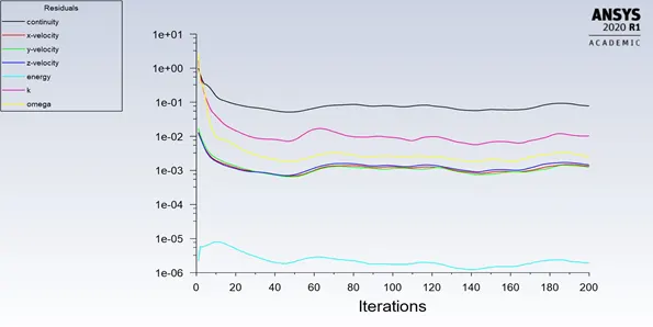
Fig: Residuals shows the convergence of the continuity and other parameters for K-omega model

8.1 HEAT TRANSFER COEFFICIENT ANALYSIS AT PLANE 1

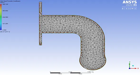
Fig: Surface HTC seen at Plane 1

Function calculator shows below the average value of the HTC in the region of Plane 1

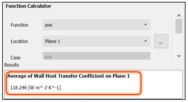
Fig: avg HTC at Plane 1

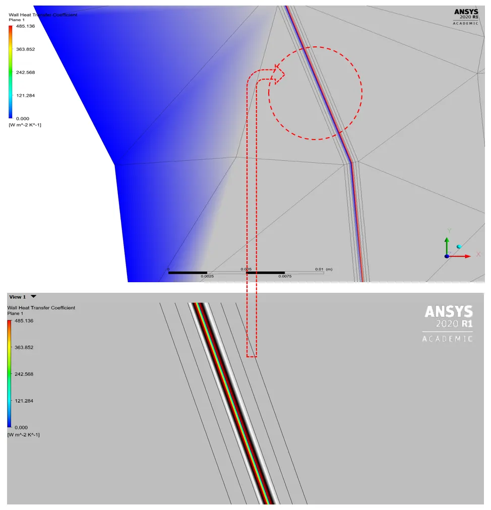
Fig: HTC at the Inflation layers Boundary in Plane 1

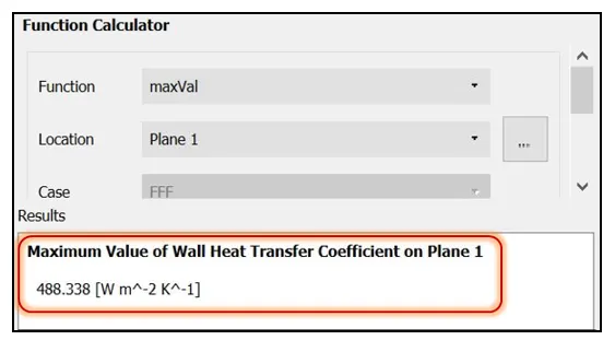
Fig: max HTC at Plane 1

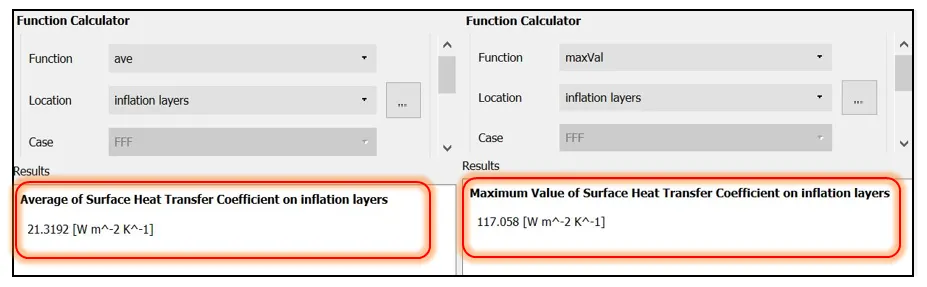
Fig: average and maximum HTC at the inflation layers

8.2 TEMPERATURE CONTOURS ANALYSIS AT PLANE 1

Fig: temperature contours at the plane 1

The temperature contours at plane 1 for the inner fluid region shows that the maximum temperature goes in some particular region only and this region starts from the curvature region after the mixing of all 4 inlet exhaust gases and till before the outlet region shown in the contour by the surface named as contour number 29 which has a near temperature about 692.327 K.

Now this can be clearly inferred from the above contour that the temperature just after mixing of the all the gases from 4 inlet ports there is a significant increase in the temperature shown by the 29^th contour which is greater than the temperature of gases just after they inter through the inlet port i.e. the regions compared from contours 15, 19, 24,25,26,21 and many more in that region.

Also this can be inferred from the outer aluminium shell interacting with the internal hot fluid that same pattern of increase in the temperature can be seen in the regions where the all fluids mix all together and the maximum temperature can be observed in the outer sold region in plane 1 at the outlet region with the temperature around 615-620 K.

8.3 VELOCITY CONTOURS ANALYSIS AT PLANE 1:

Below contour shows the velocity contour at plane 1 which clearly shows the maximum velocity region at the bends and its max value is around 37.316 m/sec the velocity before and after this region is much lesser as compared to this region. The probable reason behind this contour can be the steep (lesser radii) curve in this region and the general mass flow equation and the continuity equation altogether conserving the mass flow rate. Thus the contour in the below fig named as 29 shows the maximum velocity region as compared to the velocity just after the inlets and as compared to even outlet region.

Fig: Velocity contours at the plane 1

Fig: region with the maximum KE

The maximum value of turbulence KE for plane 1 is 41.8019 m^2s^-2

The minimum value of turbulence KE for plane 1 is 6.40051e^-6 m^2s^-2 which is too less.

Fig: value of turbulence KE in plane 1

8.4 ANALYSIS OF Y+ VALUE ALONG THE LINE 1 IN THE PLANE 1:

The below histogram for the turbulence model K omega in the region of all domain of the CAD model shows that almost more than 97% of the region shows the value of Y+ <= 5. The maximum of the region where shows the value of Y+ as 1.22-1.68 in 40%. This shows that the aim of keeping the value of Y+ in below 5 for the given model is achieved up to more than 97% for more refined inflation.

Fig: the % of Y+ value lying in the region of all domain

Fig: scatter plot of Y+ in the domain

Fig: the value of Y+ at the outlets and inflation layer shadows

Y+ VERIFICATION THEORETICALLY:

Verification for Y+ theoretically with the simulation results can be done with the use of parameters like the value of Y, the velocity at the wall region where we want to get the Y+ and the kinematic viscosity thus is related by the formula below:

Where the Y as maximum inflation layer was selected around 0.000005 m (for 3 layers each side)

Ƿ Density is considered as per the material as 1.225 kg/m^3

Velocity around 20m/sec as achieved as the avg for plane 1

µ Dynamic viscosity as around 2* 10^-5 kg/m-sec

This gives the value of Y+ as around 3 which is almost equal to the inflation layers shadows.

The value of an inflation layers are supposed to be varying from place to place depending upon the domain when we try to calculate it theoretically as it depends upon other parameters such as velocity, kinematic viscosity, the depth of inflation and the density out of which the velocity continues to vary of we move from one region to the other, the density and kinematic viscosity although remains constant and the depth depends upon as per the calculations which we achieve from the Y+ value for a particular turbulent kinematic model.

8.5 TEMPERATURE AND VELOCITY ANALYSIS ALONG THE LINE 1 IN THE PLANE 1:

Fig: line 1 along plane 1

Fig: temperature max value at line 1

As per the given domain here for the line 1 here we will discuss the plots of temperature and velocity along the line w.r.t the chart count the velocity plots and temperature plots shows the characteristics very similar to what is observed later in the contours at the other planes and streamlines

The velocity plot seen in the next plot along the line 1 shows clearly the maximum velocity region with the points defined as point 2 and which later can be verified with the streamline and the reason if it being lying in the mass conservation principle and continuity equations.

PLOTS TO JUSTIFY THE TEMPERATURE & VELOCITY VARIATION ALONG LINE 1:

The below plots shows the regions of the variation of temperature and velocity along the line 1. As per the temperature is concerned it shows high value near the sharp curvature region in the previous show contours and as per velocity it has already been shown by contours that the maximum lies at the steeper curve region and after the mixing of all the exhausts till before the inlet region. The region can be better understood as the end points are listed already inside the plots.

Fig: temperature plot vs chart count along line 1

Fig: velocity plot vs chart count along line 1

8.6 PLOTS OF PARAMETERS IN THE PLANE 2:

Below fig shows the plane 2 and following it will show the different contours that support the results for its better understandings.

Fig: plane 2 introduction

Fig: Temperature contours at plane 2

Below plots shows the much clear indications of the regions with maximum velocity which can further be seen more clearly by the path lines and streamlines functions plots.

Fig: velocity contours at plane 2

Fig: KE contours at plane 2

Below plot shows the Reynolds number contour for the fluid region in the plane 2 which goes from min 0 to maximum value of 9282.81 for the contour number 25 as seen from fig.

Fig: Re number count contours

8.7 STREAMLINES AND PATHLINES FOR VELOCITY & KE:

Fig: Side view of velocity streamlines showing the region of maximum velocity

Fig: isomeric view for the velocity streamlines

Fig: turbulence KE streamlines

PATHLINES FOR VELOCITY AND Re:

Fig: velocity path lines

Fig: Re showing highest in the region of and after the sharp bend and after mixing

8.8 TEMPERATURE ANALYSIS AT INFLATION LAYERS:

Fig: Temperature variations at the inflation layers

Fig: Max temperature at the inflation layers

8.9 TEMPERATURE AND VELOCITY ANALYSIS AT THE OUTLET:

Fig: max temp at outlet

Fig: outlet temperature contours

Fig: outlet velocity contours

Fig: outlet turbulent Re contours

Fig: outlet turbulent KE

CONCLUSION:

The CHT phenomenon has been described with its applications in the introduction of the report. Also as discussed earlier about the model used for the simulation justifies its theoretical definition when seen form the various temperature and velocity contours in different regions as per the identification is required. Various sections like plane 1, plane 2, outlet and inflation layer shadow regions has been used to discuss the behaviour of different types of parameters and variables.

As per the given problem statement the value of Y+ has been checked successfully according to the chosen turbulence model of k omega and the simulation clearly shows that the value of Y+ in the domain lies maximum in 97% region where the value of Y+ is in the range of 0-5 and which is actually been seen in the k omega model for SST for the near wall type analysis. The support for it can be seen in a much better form from the histogram and the scatter plot of Y+ as shown in the report previously.

• Verification for HTC for the plane 1 region:

The results from the simulation shows the value of the HTC is around 488 W/ (m^2-K) which when verified through the theoretical calculations as per the plane region gives the following calculation

We know that Q=h*A*ΔT

Here the value of maximum heat flux is around 14500 J/sec and the area of the plane as calculated from the function calculator in post processing is 0.1463 m^2 and the max and min temperature was seen to be 700K and 477 K . Thus

A= 0.1463 m^2

ΔT= 223 K

Q= 14500 W

This gives the value of HTC for the wall of the plane 1 equals to 444 W/ (m^2-K)

Thus the value of HTC as per the maximum value achieved from the simulation are much near and can be taken into considerations given the intricate shapes of the geometry and some values taken as per the lenient range.

Lastly the factors on which the HTC seems to depend upon are the geometry, the temperature of the flowing fluid in the region, the material properties of the fluid, the flow regime, fluid to wall temperature ratio, the velocity of the fluid flowing in the region and also on thermal factors of fluid such as the heat capacity Cp, the viscosity and other such factors. Variation in any above mentioned parameters can lead to change in the obtained HTC as per the simulation thus the boundary conditions set as per the maned parameters should be taken into considerations if we want to control the precision of the HTC for the domain of the CAD geometry.

The outlet shows that the temperature in the outlet as per contours isn’t as much high as its seen to be in the plane 1 region contour at the curve region. This shows that the temperature is here driven somehow with the magnitude of velocity in a particular region. The max temperature region is the region where the velocity is significantly high and the geometry is also somewhat curvaceous and the bend is significantly steep. This shows that the temperature depends on not only on the region close to the source but also significantly on other factors such as the geometry and the velocity and other factors.