Rankine cycle Simulator using MATLAB.

OBJECTIVE:

1. Code to calculate the state point of rankine cycle based on user inputs.
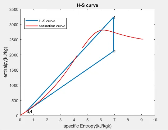
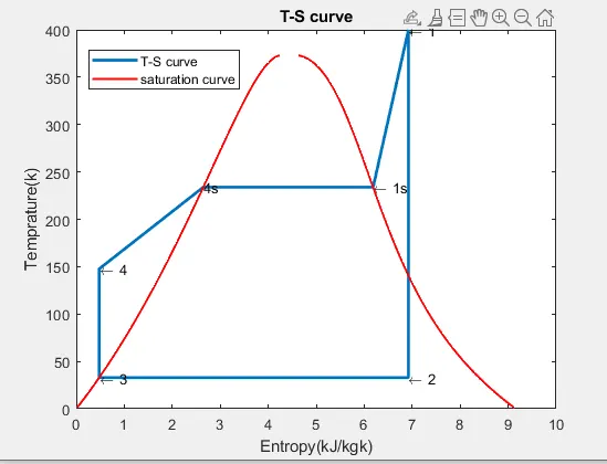
2. Plot the H-S and T-S curve.
3. Calculate the net work output and back work ratio.

RANKINE CYCLE:

The Rankine cycle or Rankine Vapor Cycle is the process widely used by power plants such as coal fired power plants ornuclear reactors. In this mechanism, a fuel is used to produceheat within a boiler, converting water into steam which then expands through a turbine producing usefu work.

components used:

1) Turbine 2)Condenser 3)Pump 4)Boiler

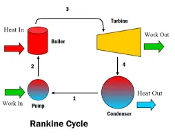
The efficiency of the Rankine cycle is limited by the high heat of vaporization by the fluid. The fluid must be cycled through and reused constantly, therefore, water is the most practical fluid for this cycle. This is not why many power plants are located near a body of water—that's for the waste heat.

As the water condenses in the condenser, waste heat is given off in the form of water vapour—which can be seen billowing from a plant's cooling towers. This waste heat is necessary in any thermodynamic cycle. Due to this condensation step, the pressure at the turbine outlet is lowered. This means the pump requires less work to compress the water—resulting in higher overall efficiencies.

process include in rankine cyce:

1-2 process: isentropic expansion in turbine.

2-3 process: constant pressure heat rejection in condenser.

3-4 process: isentropic compression using pump.

4-1 process: constant pressure heat addition in boiler.

FORMULA USED:

T4 = T1s/exp((s1f-s4)/high_cpl);

Wnet = Wt - Wp

B.W.R = -Wp/Wt

Efficiency =Wnet*100/Qin

high_cpl = specific heat constant of fluid at p1

where,

T4 = temprature at the inlet of the boiler.

T1s = temprature at the saturation line of state1

s1f = fluid entropy at the inlet of turbine

s4 = entropy of fluid at the inlet of boiler

high_cpl = specific heat constant of fluid at p1

Wnet =net workdone

B.W.R = back work ratio

Wp = work done byb pump

Wt = work done by turbin

Qin =heat addition to the fluid in boiler

CODE TO SOLVE THE CYCLE:

clear all
close all
clc

% inputs required
p1 = input('Enter the Pressure at the Turbine inlet(in bar):');  
T1 =  input('Enter The Temprature at turbine inlet:');      
p2 = input('Pressure at condenser inlet:'); 


% finding cp (specific heat constant) at p1
high_cpl = XSteam('cpL_p',p1);


%state variable at point 1
disp(' variables At state point 1:')
fprintf('p1  :%f bar\n',p1)
T1s = XSteam('Tsat_p',p1);  %temprature at saturation line
s1s = XSteam('sV_p',p1);
s1f = XSteam('sL_p',p1);
h1 = XSteam('h_pT',p1,T1);    
fprintf('h1  : %f kJ/kg \n',h1)
s1 = XSteam('s_pT',p1,T1);      
fprintf('s1  : %f kJ/kgk \n',s1)
fprintf('T1  : %f Deg celsius \n',T1)


%state variable at point 2
disp('variables at state pint 2:')
fprintf('p2  :%f bar \n',p2)
s2 = s1;
hg2 = XSteam('hV_p',p2);
hf2 = XSteam('hL_p',p2);
sg2 = XSteam('sV_p',p2);
sf2 = XSteam('sL_p',p2);
x2 = (s2-sf2)/(sg2-sf2);
h2 = hf2+x2*(hg2-hf2);
fprintf('h2  : %f kJ/kg \n',h2)
fprintf('s2  : %f kJ/kgk \n',s2)
T2 = XSteam('Tsat_p',p2);
fprintf('T2  : %f Deg celsius \n',T2)


%state variable at point3
disp('variables at state pint 3:')
p3 = p2;
fprintf('p3  :%f bar \n',p3)
hf3 = XSteam('hL_p',p3);
h3 = hf3;
fprintf('h3  : %f kJ/kg \n',h3)
sf3 = XSteam('sL_p',p3);
s3 = sf3;
fprintf('s3  : %f kJ/kgk \n',s3)
T3 = T2;
fprintf('T3  : %f Deg celsius \n',T3)

%state variable at point 4
disp('variables at state pint 4:')
p4 = p1;
fprintf('p4  :%f bar \n',p4)
s4 = s3;
hf4 = XSteam('h_ps',p4,s4);
h4 = hf4;
fprintf('h4  : %f kJ/kg \n',h4)
fprintf('s4  : %f kJ/kgk \n',s4)
T4 = T1s/exp((s1f-s4)/high_cpl);
fprintf('T4  : %f Deg celsius \n\n',T4)

T5 = T1s;
s5 = XSteam('sL_T',T5);

%plotting H-S curve
figure(1)
plot([s1 s2 s3 s4,s1],[h1 h2 h3 h4 h1],'linewidth',2)
xlabel('specific Entropy(kJ/kgk)')
ylabel('enthalpy(kJ/kg)')
title('H-S curve')
text(s1,h1,'1')
text(s2,h2,'2')
text([s3 s4],[h3 h4],'3,4')
hold on

% creating saturation line
Tc = linspace(1,373,500);
for i = 1:length(Tc)
    %saturated-liquid line 
    hl(i) = XSteam('hL_T',Tc(i));
    sl(i) = XSteam('sL_T',Tc(i));
    %saturated vapour line
     hv(i) = XSteam('hV_T',Tc(i));
    sv(i) = XSteam('sV_T',Tc(i));
        
end
%plotting saturation line
plot(sl,hl,'r','linewidth',1.5)
plot(sv,hv,'r','linewidth',1.5)
legend('H-S curve','saturation curve')
    

figure(2)
plot([s1 s2 s3 s4 s1f s1s s1],[T1 T2 T3 T4 T5 T1s T1],'linewidth',2)
xlabel('Entropy(kJ/kgk)')
ylabel('Temprature(k)')
title('T-S curve')
text(s1,T1,'\leftarrow 1')
text(s2,T2,'\leftarrow 2')
text(s3,T3,'\leftarrow 3')
text(s4,T4,'\leftarrow 4')
text(s1s,T1s,'\leftarrow 1s')
text(s1f,T5,'4s')
hold on

% plot for saturation line
plot(sl,Tc,'r','linewidth',1.5)
plot(sv,Tc,'r','linewidth',1.5)
legend('T-S curve','saturation curve')

%work done by the turbine
Wt = h1 - h2;

%work done by pump
Wp = h4 -h3;

%net work
Wnet = Wt-Wp;
fprintf('net work : %f kJ/kg \n', Wnet)

%back work ratio
B.W.R = -Wp/Wt;
fprintf(' back work ratio : %f  \n', B.W.R)

%heat addition
Qin = h1 - h4;

% thermal efficiency
TE = Wnet*100/Qin;
fprintf('thermal efficiency  : %f percent ', TE)

EXPLANATION OF THE CODE :

1. First of all, set the input variables p1, T1, and p2 using input command.
2. Calculating the variables at state 1,2, 3 and 4 state using the XSteam which is having all values of steam table file.
3. Plot the H-S curve using plot command.
4. The saturation curve can be plotted by dividing the temprature into parts upto 373kelvin(which is critical temprature of water) and finding the value of enthaly and Entropy for liquid and vapour for the abouve defiend range of temprature.
5. Plot the saturattion line using plot command.
6. Plotting T-S curve and saturation curve in figure 2
7. Calculating net work , backwork ratio and efficiency using the above formulas.

ERROR FACED:

Fortunately whole the project was on track and no errors faced while executing the prgram.

OUTPUT:

output in command window:

Enter the Pressure at the Turbine inlet(in bar):30
Enter The Temprature at turbine inlet:400
Pressure at condenser inlet:0.05
 variables At state point 1:
p1  :30.000000 bar
h1  : 3231.571027 kJ/kg 
s1  : 6.923259 kJ/kgk 
T1  : 400.000000 Deg celsius 
variables at state pint 2:
p2  :0.050000 bar 
h2  : 2110.708212 kJ/kg 
s2  : 6.923259 kJ/kgk 
T2  : 32.875490 Deg celsius 
variables at state pint 3:
p3  :0.050000 bar 
h3  : 137.765119 kJ/kg 
s3  : 0.476254 kJ/kgk 
T3  : 32.875490 Deg celsius 
variables at state pint 4:
p4  :30.000000 bar 
h4  : 140.762226 kJ/kg 
s4  : 0.476254 kJ/kgk 
T4  : 147.599058 Deg celsius 

net work : 1117.865709 kJ/kg 
 back work ratio : -0.002674  
thermal efficiency  : 36.167417 percent 

H-S PLOT:

T-S PLOT:

REFRENCES:

1. https://energyeducation.ca/encyclopedia/Rankine_cycle#:~:text=The%20Rankine%20cycle%20or%20Rankine,a%20turbine%20producing%20useful%20work.