PV diagram of air standard Otto Cycle using Matlab

AIM - Draw a PV diagram of air standard otto cycle using Matlab.

Objectives –

To write code in Matlab and that can solve an otto cycle and Plot PV Diagram.
The code should create a PV diagram.
Finding the thermal efficiency of the engine.

Basics –

1. Otto cycle- Air standard Otto cycle is used for the SI Engines. The cycle Contains Mainly four Processes. In the overall cycle, suction and Exhaust are neglected, also power consumption is not considered.
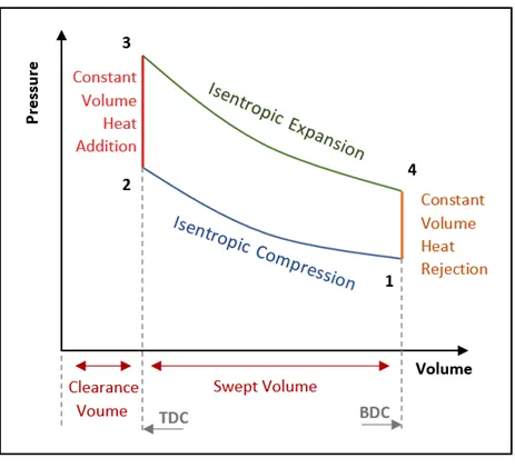
The Ideal Oto cycle consists of the four processes which are as below.

1–2 Reversible Adiabatic compression (Or) Isentropic Compression.
2–3 Constant Volume Heat Addition.
3–4 Reversible Adiabatic Expansion (Or) Isentropic Expansion.
4–1 Constant Volume Heat Rejection.

When the piston in the cylinder of the Internal Combustion Engine (SI Engine) moves from BDC (i.e Bottom Dead Centre) to TDC (i.e Top Dead Centre) the Pressure and volume Relatively change, which is represented on the Diagram known as PV-Diagram.

2. Compression ratio (cr):- It is the ratio of volume before compression to the volume after compression.

Compression ratio (cr) = Volume before compression/volume after compression

also, Compression ratio (cr) = (Vs+Vc)/(Vc)

Where-

v1= volume before compression = v_swept + v_clearance

v2 = volume after compression = v_clearance

vs = v_swept , vc = v_clearance

Therefore, Compression ratio (cr) = (v1)/(v2)

3. Expansion ratio (er):- It is the ratio of volume after Expansion to the volume before compression.

Similarly, as the compression ratio, we can get an Expansion ratio.

Therefore, Expansion ratio (er) = (v4)/(v3)

for Otto cycle compression Ratio = Expansion ratio i.e (cr=er)

3. Swept volume and Clearance volume:- Swept Volume (v_s) is a volume Before compression stroke. Also known as stoke volume and Displacement volume. Similarly, Clearance volume (v_c) is a volume after compression stroke.

Now calculate state variables at point 1

Initial Pressure & Temperature:

P1= 101325 bar, T1= 500 K

1. Engine Geometry parameters:

   Bore (D) = 0.1 m

   Stroke (L) = 0.1 m

   Connceting rod Length (con_rod) = 0.15 m

   And Compression Ratio (cr) = 12

   gamma = 1.4

2. Swept volume and Clearance volume

Clearance volume v_c = v_s/(cr-1)

Swept Volume v_s = (pi/4)*D²*L ( D is bore and L is stroke length)

Now calcululate state variable at point 2

Calculating Pressure at point 2 (p2)

Due to isentropic compression, we can apply the PV Relation here.

p1v1^gamma = p2v2^gamma

Where, p2 is Unkown to us which can be calculated with the help of the relation between the volume, pressure and compression ratio

Also, we can calculate the p2 as follow

Cr = v1/v2 = (p2/p1)^gamma

Therefore, p2 = p1 * ( cr )^gamma

Calculating temp at point 2 (t2)-

To get the value of temp t2 we are using the ideal gas equation as follows.

p1v1 = mRt1 , mR = p1v1/t1

p2v2 =mRt2 , mR = p2v2/T2

Therefore, p1v1/T1 = p2v2/t2

Hence, t2 = p2*v2*(t1)/(p1*v1)

Now calculate state variables at point 3

Calculating Volume at point 3 (v3)

v3=v2

Calculating Pressure at point 3 (p3)

By using the ideal gas equation

p3 = p2 * (t3)/(t2)

Now calculate state variables at point 4

Calculating Volume at point 4 (v4)

v1= v4

Calculating Pressure at point 3 (p3)

Also from p3v3^gamma = p4v4^gamma.

p4 = p3 *[(v3)/(v4)]^gamma

we have all values so we can plot the pv curve and calculate Percentage Efficiency

thermal efficiency= (1-(cr^(gamma-1))^-1)*100

Procedure and Explanation for Matlab

clear all
close all
clc

%state variables
p1 = 101325
t1 = 500
gamma = 1.4 
t3 = 2300

%engine geometric parameters
bore = 0.1;
stroke = 0.1;
con_rod = 0.15;
cr = 12;

%calculating swept volume and clearance volume
v_swept = (pi/4)*bore^2*stroke;
v_clearance = v_swept/(cr-1);
v1 = v_swept + v_clearance
v2 = v_clearance

% state variables at state point 2
% p2v^gamma = p1v1^gamma
% p2 = p1*(v1/v2)^gamma = p1*c^gamma
p2 = p1*cr^gamma;
% p1v1/t1 = p2v2/t2 | t2=p2*v2*t1/(p1*v1)
t2 = p2*v2*t1/(p1*v1);

% state varianles at state point 3
v3 = v2
% p3v3t3 = p2v2/t2 | p3 = p2*t3/t2
p3 = p2*t3/t2


 % state variables at state point 4
 v4 = v1
 % p3v3^gamma = p4v4^gamma | p4 = p3(v3/v4)^gamma
 p4 = p3*(v3/v4)^gamma

 

 figure(1)
 hold on 
 plot(v1,p1,'*','color','r')
 plot(v2,p2,'*','color','r')
 plot(v3,p3,'*','color','r')
 plot(v4,p4,'*','color','r')

 xlabel('Volume (m^3)')
 ylabel('Pressure (KPa)')

Where:-

Clear all command used to clear text from the Command Window before running a command.

Close all command used to close all the plots window.

clc command is used to Clear Command Window

The input and state points are taken as discussed.

For plotting, we are using plot command and we get a PV diagram having four-point in it which Represents State points. after Executing the Program we get our required output as

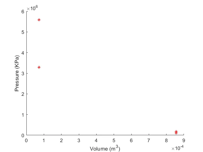
now we have all points so lets connect them. but We cannot join them form line because isentropic processes do not have constant slope. If we try, we get the result as follows by using the following command, which is an Error.

plot([v1 v2 v3 v4 v1],[p1 p2 p3 p4 p1],'color','r')

clear all
close all
clc

%state variables
p1 = 101325
t1 = 500
gamma = 1.4 
t3 = 2300

%engine geometric parameters
bore = 0.1;
stroke = 0.1;
con_rod = 0.15;
cr = 12;

%calculating swept volume and clearance volume
v_swept = (pi/4)*bore^2*stroke;
v_clearance = v_swept/(cr-1);
v1 = v_swept + v_clearance
v2 = v_clearance

% state variables at state point 2
% p2v^gamma = p1v1^gamma
% p2 = p1*(v1/v2)^gamma = p1*c^gamma
p2 = p1*cr^gamma;
% p1v1/t1 = p2v2/t2 | t2=p2*v2*t1/(p1*v1)
t2 = p2*v2*t1/(p1*v1);

% state varianles at state point 3
v3 = v2
% p3v3t3 = p2v2/t2 | p3 = p2*t3/t2
p3 = p2*t3/t2


 % state variables at state point 4
 v4 = v1
 % p3v3^gamma = p4v4^gamma | p4 = p3(v3/v4)^gamma
 p4 = p3*(v3/v4)^gamma

 

 figure(1)
 hold on 
 plot(v1,p1,'*','color','r')
 plot(v2,p2,'*','color','r')
 plot(v3,p3,'*','color','r')
 plot(v4,p4,'*','color','r')
plot([v1 v2 v3 v4 v1],[p1 p2 p3 p4 p1],'color','r')
 xlabel('Volume (m^3)')
 ylabel('Pressure (KPa)')

we get these error

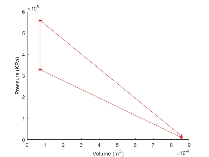
these curve is completely wrong so we need to eliminate error.

To plot correctly, we need the following two things.

1. Thermodynamic relation during compression
2. Piston kinematics to determine How the volume change from TDC to BDC and how combustion volume changes as a function of the crank angle.
3. basically we need to create functon

codes for create function

function [V] = engine_specifications(bore, stroke, con_rod, cr, start_crank, end_crank)

 a = stroke/2
 R = con_rod/a;
 v_s = (pi/4) * bore^2 * stroke
 v_c = v_s/(cr-1)
 
 theta = linspace(start_crank,end_crank,100);
 
 %formula
 term1 = 0.5*(cr-1);
 term2= R+1-cosd(theta);
 term3 =(R^2-sind(theta).^2).^0.5;
 
 V = (1+term1*(term2-term3)).*v_c;
end

Here, we are taking all the parameters same as above but we need a different formula for the calculation of the volume change inside the combustion chamber. The required relationship we can get by the following formula.

v/vc = 1+ 0.5(cr-1)* [ R+1 -cosd(theta) — (R² -sind²(theta)^0.5]

To simplify the formula we divided formula into three sub formulas as follows

term1 = 0.5*(cr-1);
term2= R+1-cosd(theta);
term3=(R²-sind²(theta))^0.5;

At last, we get our final formula as

V=(1+term1*(term2-term3))*v_c

Where:-

R= Length of connecting rod/Crankpin radius

Now, we are going to use this Program in our first program for getting PV Diagram correctly, But using total program to our first program is non-convenient therefore we are introducing the predefine command in Matlab known as function, which is a piece of code that we can read by calling its name.

Function [V] =engine_specifications(bore,stroke,con_rod,cr,start_crank,end_crank)

we need to take care of function name and file name should be same and there location should be in same folder.

calculate V_compression by calling fuction

so V_compression = engine_specifications(bore,stroke,con_rod,cr,180,0);

But for the pressure, we know that p*v^gamma = constant

Hence, we are defining this relation and using it as, constant_c = p1*v1^gamma; and P_compression = constant_c./V_compression.^gamma;

similarly, for Expansion, we are using the above relation as,

constant_c = p3*v3^gamma;
V_expansion = engine_specificatons(bore,stroke,con_rod,cr,180,360);
P_expansion = constant_c./V_expansion.^gamma

Calculate thermal efficiency

use formulae

thermal efficiency = (1-(cr^(gamma-1))^-1)*100

to run the program make sure that your main program and fuction in same folder its mandatory.

onc do this our main program look like this

Final Matlab Program

clear all
close all
clc

%state variables
p1 = 101325
t1 = 500
gamma = 1.4 
t3 = 2300

%engine geometric parameters
bore = 0.1;
stroke = 0.1;
con_rod = 0.15;
cr = 12;

%calculating swept volume and clearance volume
v_swept = (pi/4)*bore^2*stroke;
v_clearance = v_swept/(cr-1);
v1 = v_swept + v_clearance
v2 = v_clearance

% state variables at state point 2
% p2v^gamma = p1v1^gamma
% p2 = p1*(v1/v2)^gamma = p1*c^gamma
p2 = p1*cr^gamma;
% p1v1/t1 = p2v2/t2 | t2=p2*v2*t1/(p1*v1)
t2 = p2*v2*t1/(p1*v1);
constant_c = p1*v1^gamma;
V_compression = engine_specifications(bore,stroke,con_rod,cr,180,0);
P_compression = constant_c./V_compression.^gamma;
% state varianles at state point 3
v3 = v2
% p3v3t3 = p2v2/t2 | p3 = p2*t3/t2
p3 = p2*t3/t2
constant_c = p3*v3^gamma;
V_expansion = engine_specifications(bore,stroke,con_rod,cr,180,360);
P_expansion = constant_c./V_compression.^gamma;

 % state variables at state point 4
 v4 = v1
 % p3v3^gamma = p4v4^gamma | p4 = p3(v3/v4)^gamma
 p4 = p3*(v3/v4)^gamma

 % thermal efficiency
 
 Percentage_Efficiency = (1-(cr^(gamma-1))^-1)*100


 figure(1)
 hold on 
 plot(V_compression,P_compression,'linewidth',1.5,'color', 'b')
 plot(V_expansion,P_expansion,'linewidth',1.5,'color', 'b' )
 plot([v2 v3],[p2 p3],'linewidth',1.5,'color', 'g')
 plot([v4 v1],[p4 p1],'linewidth',1.5,'color', 'g')

 plot(v1,p1,'*','color','r')
 plot(v2,p2,'*','color','r')
 plot(v3,p3,'*','color','r')
 plot(v4,p4,'*','color','r')
 xlabel('Volume (m^3)')
 ylabel('Pressure (KPa)')

Where:-

Plot Command is used to get the final plot but we need to plot the two graphs in the same figure. so we are using subplot command to do it.

xlable and ylabel command used to define the labels in the plots. title command is used to define the plot title.

our output graph is below

Our output pv diagram

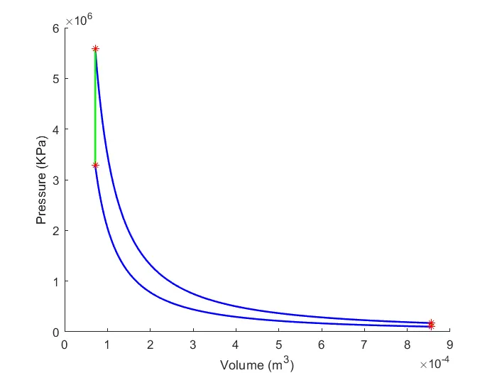
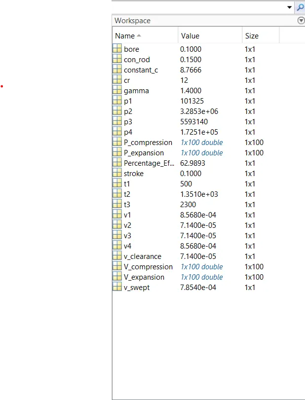
Our all Variables and their valus.

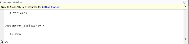
Our Effficiency-

Thanks.....