Curve Fitting Using Matlab
Aim-
To write a code for to fit a linear and cubic polynomial for the Cp data and to show splitwise method using matlab
Basic theory of Curve Fit-
Curve fitting is the process of constructing a curve, or mathematical function, that has the best fit to a series of data points, possibly
subject to constraints. Curve fitting can involve either interpolation, where an exact fit to the data is required, or smoothing, in which a" smooth" function is constructed that approximately fits the data. A related topic is regression analysis, which focuses more on
questions of statistical inference such as how much uncertainty is present in a curve that is fit to data observed with random errors.
Fitted curves can be used as an aid for data visualization, to infer values of a function where no data are available, and to summarize
the relationships among two or more variables. Extrapolation refers to the use of a fitted curve beyond the range of the observed
data, and is subject to a degree of uncertainty since it may reflect the method used to construct the curve as much as it reflects the
observed data.
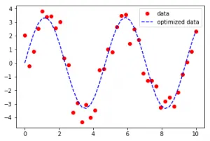
1. To find a curve fit for the given data points there are many methods, since our aim is to find curve fit for a linear and cubic
polynomial the most common way to fit curves to the data is using regression method. Typically, you choose the model order
by the number of bends you need in your line. Each increase in the exponent produces one more bend in the curved fitted
line.
2. After finding the curve which satisfies the data points, there are four quantities which help us measure the goodness of fit
criteria or how well the equation is a representing the data points.
3. For goodness of fit, we are using least square method which is the most common method as long as fitting curve is a
polynomial
4. These quantities are:
i) The sum of squares due to error (SSE)
ii) R-square
iii) Adjusted R-square
iv) Root mean squared error (RMSE)
5. SSE: This statistic measures the total deviation (i.e. error) of the data points from the curve fit[y= f(x)] to the data points. It is also
called the sum of squares of due to error. and is usually labeled as SSE.
The error for a general “i” point can be given by the function,
Error = |y(i) − value of f(x) at x(i)| = |y(i) − f(x(i))|
To remove the modulus sign, it is effective if we square the error term, when we square the error terms and add the errors
for all the ‘n’ points we get,

A value closer to 0 indicates a better fit.
6. R-square: This statistic measures how successful the fit is in explaining the variation of the data. Put another way, R-square is
the square of the correlation between the data points and the predicted data points. It is also called the square of the multiple
correlation coefficient and the coefficient of multiple determination.
R-square is defined as the ratio of the sum of squares of the regression (SSR) and the total sum of squares (SST).
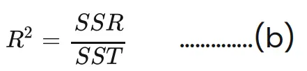
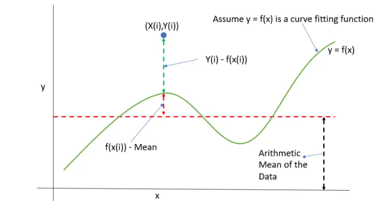
SSR= it is the square of the difference between the values of the fitting function at a given point and the arithmetic mean of
the data set

Now SST is given as,
SST = SSR + SSE ...........(d)
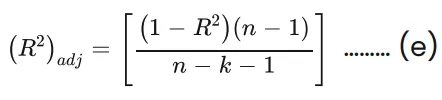
7. Adjusted R-square: It is a normalizing variation of R-square which neglects the variation of R-square due to insignificant
dependent variables.
Let y = f(x) then,
If value of x(i) contributes to the output y, then x(i) is a significant dependent variables.
If value of x(i) does not contribute to the output y, then x(i) is an insignificant dependent variables.
So , Adjusted R-square disregards these infinitesimally small increments to R-square, and only considers the variables which
actually contribute to the output of the system in a drastic way
Where,
n = number of data points
k = number of independent variables
The adjusted R-square statistic can take on any value less than or equal to 1, with a value closer to 1 indicating a better fit.
8. RSME: This statistic is also known as the fit standard error and the standard error of the regression. It is the distance from the
fitted curve to the data points.
If this distance is less it is considered good fit.
If this distance is more it not considered good fit.

Where ,
n is the total number of data points available.
RMSE value closer to 0 indicates a better fit.
Note - all theory is from mathwork community.
Now Matlab Program For Linear fit Curve
clear all
close all
clc
cp_data = load('data');
temperature = cp_data(:,1);
cp = cp_data(:,2);

%cp = a*t+c
co_effs = polyfit(temperature,cp,1);
predicted_cp = polyval(co_effs,temperature);
%Plotting
plot(temperature,cp,'linewidth',3)
hold on
plot(temperature, predicted_cp,'linewidth',3,'color','r')
xlabel('Temperature [K]')
ylabel('Specific Heat [KJ/Kmol-K]')
axis([0 4000 900 1500]);
title('Linear Polynomial Curve Fit')
legend('Original Dataset','Curve Fit')
%Calculation for Goodness of curve
for i=1:length(cp);
 x(i)=(predicted_cp(i)- cp(i))^2;
 y(i)=(predicted_cp(i)- mean(cp))^2;
end
SSE= sum(x);
SSR= sum(y);
k=0;
n=3200;
R_square= (SSR/(SSE+SSR));
a = (1- R_square)*(n-1);
b = (n-k-1);
Adjusted_R_square = 1-(a/b);
RSME= (SSE/length(temperature))^0.5;
EXPLANATION:
1. First the program is started with ‘clear all’, ‘close all’, ‘clc’ and then a data file is loaded using the ‘load()’ command to load the
file that is named as ‘data’. This data should be in the same folder where the main code is saved.
2. Now when you run the code after using the ‘load()’ command you will see a (3200 x 2) matrix in the workspace.
1. Once you see this matrix in workspace, which will ensure us that we have loaded the correct data file.
2. This loaded data is assigned to a variable ‘cp_data’.
3. Since the first column of the data set are the values of temperature so it is assigned to a variable ‘temperature’.
4. Similarly second column of data set are the values of specific heat so it is assigned to a variable ‘cp’.
5. Now let us assume that a linear polynomial cp=at+c is a curve that fits the original data points where ‘t’ and ‘cp’ are variables.
So to find the polynomial we need to fine the values of co-efficients ‘a’ and ‘c’.
6. To find value of co-efficients ‘polyfit()’ command is used.
7. Syntax for ‘ployfit()’ command is ,
8. p = polyfit(x,y,n),
9. p = polyfit(x,y,n) returns the coefficients for a polynomial p(x) of degree n that is a best fit for the data in y.
10. Now in our code, ‘x’ is the temperature values and ‘y’ is the cp values and since we finding first order equation ‘n’ is one. Thus
accordingly we have entered the ‘polyfit()’ command. Since values of ‘p’ are coefficients so we have named ‘co_effs’ instead of
‘p’ in the above code. This co-efficients are thus used to find the polynomial.
11. Thus polynomial is found and now to evaluate the polynomial using above co-efficients we have used a command ‘polyval()’
and syntax for this command is,
y = polyval(p,x)
y = polyval(p,x) evaluates the polynomial p at each point in x.
12. Here since our ‘x’ is the temperature and ‘p’ is the co-efficients i.e. ‘co_effs’ in our code, so it is entered accordingly. Now we will
get values of the new cp i.e. named as ‘predicted_cp’ in the code, which are predicted values of specific heat for each and
every temperature value using the linear polynomial.
13. Then ‘plot()’ command is used to plot values of original cp and temperature and to plot the values of predicted cp and
temperature values. A ‘hold on’ command is used to prevent the overwriting of ‘plot()’ command.
14. A ‘xlabel()’, and ‘ylabel()’ commands are used to label the axis , ‘axis()’ command is used to define the limits of the x-axis and y-axis, ‘title()’ command is used to define the title of the graph, ‘legend()’ command is used to different both the curves in the
graph, Now when you run the code we can see a graph representing both the curves.
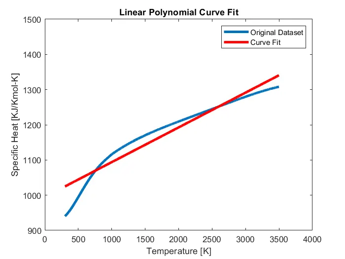
15. Above image shows us the original dataset curve and the curve fit, thus we can see that the curve fit is not fitting correctly to the
original data set. So as said above to get bends we have increase the order of the curve.
16. To check the goodness of the curve we have entered the above equations for the sum of squares due to error (SSE), R-square,
Adjusted R-square, Root mean squared error (RMSE) in the above code
17. In order to find the errors, we have used FOR LOOP , in order to find total value of SSE and SSR first we have found the SSR and SSE
for each value of cp using FOR LOOP , and SSE and SSR for each value are named as ‘x’ and ‘y’ respectively and their formula is
defined.
18. Now after the FOR LOOP is executed total SSE and SSR are calculated by adding the values of ‘x’ and ‘y’ buy using ‘sum()’
command.
19. After entering the above equations and running the code we will get the value of these terms in the workspace or in the
command window
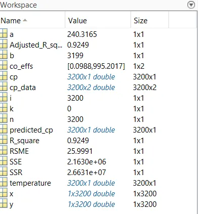
20. From the above image we can see the values of the sum of squares due to error (SSE), R-square, Adjusted R-square, Root mean
squared error (RMSE). Here value of R-square is 0.9249 which is considered not to be good and value of RSME is also very large
that means the data points very far away from the curve fit. So by increasing the order of polynomial, we can obtain good value
of these quantities.
CODE FOR CUBIC FIT CURVE
clear all
close all
clc
cp_data = load('data');
temperature = cp_data(:,1);
cp = cp_data(:,2);

%cp = a*t+c
co_effs = polyfit(temperature,cp,3);
predicted_cp = polyval(co_effs,temperature);
%Plotting
plot(temperature,cp,'linewidth',3)
hold on
plot(temperature, predicted_cp,'linewidth',3,'color','r')
xlabel('Temperature [K]')
ylabel('Specific Heat [KJ/Kmol-K]')
axis([0 4000 900 1500]);
title('Cubic Polynomial Curve Fit')
legend('Original Dataset','Curve Fit')
%Calculation for Goodness of curve
for i=1:length(cp);
 x(i)=(predicted_cp(i)- cp(i))^2;
 y(i)=(predicted_cp(i)- mean(cp))^2;
end
SSE= sum(x);
SSR= sum(y);
k=0;
n=3200;
R_square= (SSR/(SSE+SSR));
a = (1- R_square)*(n-1);
b = (n-k-1);
Adjusted_R_square = 1-(a/b);
RSME= (SSE/length(temperature))^0.5;
EXPLANATON:
1. The code for cubic fit is same that as the previous code ,the only change is that , in ‘ployfit()’ command the order is changed to
3 i.e. value of ‘n’ in syntax of ‘ployfit()’ command ,as we need a cubic fit curve.
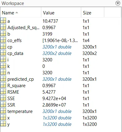
2. After the code is executed we get following graph and the values of the sum of squares due to error (SSE), R-square, Adjusted R-square, Root mean squared error (RMSE) are determined.
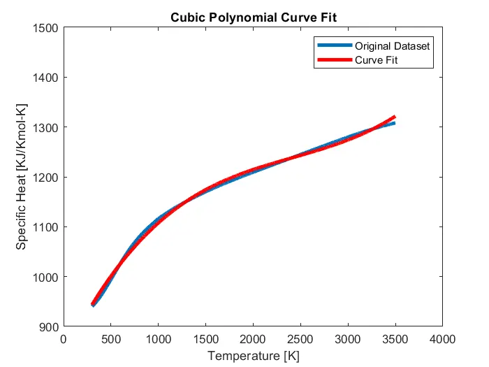
3. From above image we can observe that as we increased the order of polynomial, the curve fit is fitting more with the original
data set than compared to the linear curve.
4. When look at the values of the sum of squares due to error (SSE), R-square, Adjusted R-square, Root mean squared error (RMSE),
they are much better than that of first order polynomial. We can observe that value of R-square is 0.9962 which is good value
and RSME value is much less when compared to first order polynomial.
5. If we further increase the order of the polynomial we will get R-sqaure value near to 1 and value of RSME close to zero, which will
be near to a perfect fit.
6. But when we execute the above code we will get a warning in the Command window. Following diagram show us the error

7. This warning "Badly conditioned" means that the solution of the system of equations critically depends on rounding errors due to
the limited precision.
8. A valid solution is the centering and scaling i.e. to transform the polynomial such that the X-values have a mean of 0 and a
standard deviation (or range) of 1.
9. In Matlab we can do this centering and scaling by using ‘polyfit()’ command but with a changed syntax of the command
Checking values using Curve Fit tolbox
1. Curve fitting tool is a Matlab inbuit application where we can find the curve fit without entering any code.
2. Appropriate inputs should be given in order for this application to give correct output.
3. To open this curve fitting tool, we can type ‘cftool’ in the command window or go to ‘APPS’ in the menu bar of the Matlab, there
you will find ‘Curve Fitting’ , by clicking this a curve fiiting tool will open.
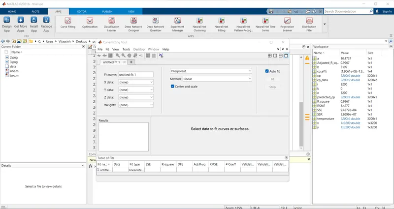
4. As we can see that in the curve fitting tool first we can give a file name then we have to select the X data and Y data an if the
data is 3-D we can also enter the Z data.
5. In the ‘Method’ option you can select the degree of polynomial and above this option we have select which type of curve fit we
need, here in our problem its polynomial curve fit.
6. We can centre and scale the curve fit automatically just by checking in the box.
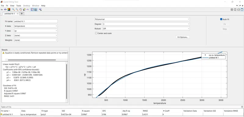
7. In Figure. we can see that after entering the inputs, the curve fitting tool automatically generates a curve fit and goodness of
curve is calculated automatically, even the coefficients of the polynomial are also calculated.
8. This tool is can be used to check our code results and verify that entered code id correct or not. Now when you compare the
code results and the curve fitting tool results ,both are equal so our code is correct.
9. Here also we can observe the same warning that had occurred ,while using a 3 degree polynomial, to eliminate this by
checking in the centre and scaling box like in Figure.13 ,automatically centering an scaling will be done and applied on the
curve fit curve.
10. So by using this tool we can generate a curve fit for the given data or we can cross check our results with this tool.
CODE FOR SPLIT-WISE METHOD-
clear all
close all
clc
cp_data = load('data');
temp = cp_data(:,1);
temp1 = temp(1:800);
temp2 = temp(801:1600);
temp3 = temp(1601:2400);
temp4 = temp(2401:3200);
cp = cp_data(:,2);
cp1 = cp(1:800);
cp2 = cp(801:1600);
cp3 = cp(1601:2400);
cp4 = cp(2401:3200);
%First Set
[co_eff_1,S1,mu1] = polyfit(temp1 , cp1, 3);
predicted_cp1= polyval(co_eff_1 , temp1,S1,mu1);
for i=1:length(cp1);
 x1(i)=(predicted_cp1(i)- cp1(i))^2;
 y1(i)=(predicted_cp1(i)- mean(cp1))^2;
end
SSE_1 = sum(x1);
SSR_1= sum(y1);
R_square_1= (SSR_1/(SSE_1+SSR_1));
RSME_1= (SSE_1/length(temp1))^0.5;
%Second Set
[co_eff_2,S2,mu2]= polyfit(temp2,cp2,3);
predicted_cp2= polyval(co_eff_2,temp2,S2,mu2);
for i=1:length(cp2);
 x2(i)=(predicted_cp2(i)- cp2(i))^2;
 y2(i)=(predicted_cp2(i)- mean(cp2))^2;
end
SSE_2= sum(x2);
SSR_2= sum(y2);
R_square_2= (SSR_2/(SSE_2+SSR_2));
RSME_2= (SSE_2/length(temp2))^0.5;
%Third Set
[co_eff_3,S3,mu3]= polyfit(temp3,cp3,3);
predicted_cp3= polyval(co_eff_3,temp3,S3,mu3);
for i=1:length(cp3);
 x3(i)=(predicted_cp3(i)- cp3(i))^2;
 y3(i)=(predicted_cp3(i)- mean(cp3))^2;
end
SSE_3= sum(x3);
SSR_3=sum(y3);
R_square_3= (SSR_3/(SSE_3+SSR_3));
RSME_3= (SSE_3/length(temp3))^0.5;
%Fourth Set
[co_eff_4,S4,mu4]= polyfit(temp4,cp4,3);
predicted_cp4= polyval(co_eff_4,temp4,S4,mu4);
for i=1:length(cp4);
 x4(i)=(predicted_cp4(i)- cp4(i))^2;
 y4(i)=(predicted_cp4(i)- mean(cp4))^2;
end
SSE_4= sum(x4);
SSR_4= sum(y4);
R_square_4= (SSR_4/(SSE_4+SSR_4));
RSME_4= (SSE_4/length(temp4))^0.5;
%Overall Result
R_Square_overall=(R_square_1+R_square_2+R_square_3+R_square_4)/4;
RSME_overall= (RSME_1+RSME_2+RSME_3+RSME_4)/4;
% Plotting
plot(temp,cp,'linewidth',6,'color','b')
hold on
plot(temp1,predicted_cp1,'linewidth',3,'color','y')
hold on
plot(temp2,predicted_cp2,'linewidth',3,'color','g')
hold on
plot(temp3,predicted_cp3,'linewidth',3,'color','m')
hold on
plot(temp4,predicted_cp4,'linewidth',3,'color','c')
xlabel('Temperature [K]')
ylabel('Specific Heat [KJ/Kmol-K]')
axis([0 4000 900 1500])
title('Split-Wise Method')
legend('original','first set curve','second set curve','third set curve','fourth set curve')
EXPLANATION:
1. In split-wise method, first the data is split into equal parts and then for each part the polynomial co-efficients are determined
and then the polynomial is calculated as it is done in the previous codes.
2. In the above code we have divided the data into 4 equal sets and given them names as ‘temp1’ , ‘temp2’ , ‘temp3’ , ‘temp4’ and
‘cp1’ , ‘cp2’ , ‘cp3’ , ‘cp4’.
3. For each set we have used ‘polyfit()’ and ‘polyval()’ command to find the co-efficients of polynomial and for computing the
polynomial.
4. For each set we have used FOR LOOP to find error for each value in that particular set and then values of the sum of squares due
to error (SSE), R-square, Adjusted R-square, Root mean squared error (RMSE) are determined.
5. Then to find the overall R-square, Adjusted R-square, Root mean squared error (RMSE) values, we have taken average of Rsquare, Adjusted R-square, Root mean squared error (RMSE) value of all the sets.
6. Then ‘plot()’ command is used to generated curves for each set and it is compared with the original data set curve.
7. ‘Hold on’ command is used to avoid the overwriting of ‘plot()’ command, ‘axis()’ comaand is used to define the limits of x-axis
and y-axis, ‘label()’ command is used to differentiate the curves in the graph.
8. Now when you run the program , the graph obtained will be much smoother than the same order polynomial graph that is
obtained without splitting the data.
9. Values are R-square, Adjusted R-square, Root mean squared error (RMSE) are also much better than the previous values
obtained without splitting the data
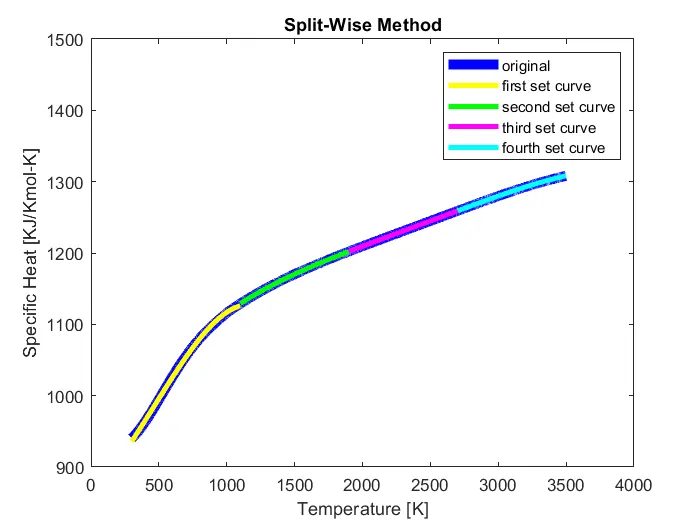
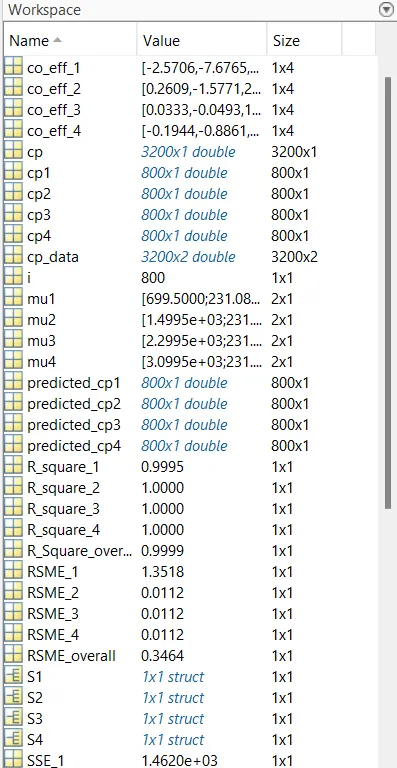
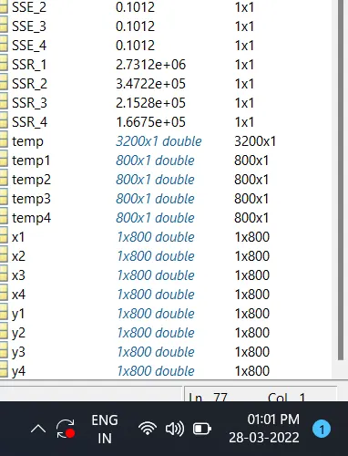
10. By comparing Figure.15 and Figure.16 we can observe that the values of R-square, Adjusted R-square, Root mean squared error
(RMSE) have improved a lot.
11. Since these value have improved, the graph in figure. is much more smooth and better than the previous one.
12. Better values can be obtained if the data set is further divided into more number of equal sets. More the number of equal sets,
more accurate will be the value.
CONCLUSIONS:
1. Thus a code for to fit a linear and cubic polynomial for the Cp data is executed successfully and the use of split wise method is
also explained.
2. Similar approach can be used for other curve fits to predict any kind of data.
3. Using split-wise method will give more goodness of the curve.
References-
All Theory is from mathworks community
https://in.mathworks.com/help/matlab/math/example-curve-fitting-via-optimization.html
https://in.mathworks.com/help/curvefit/fit.html?s_tid=doc_ta