Project - Speed Control of a Direct Current (DC) motor
In this project, a Simulink model for the DC motor will be first developed per the schematic shown in Figure 1.
Use the Proportional, Integral, and Derivative (PID) control design knowledge gained in the training to design, develop and test a controller to maintain a desired speed for the motor.
Sol:
-> Here, we need to first understand working of DC machine in detail. DC machine can be used as a Motor and Generator.
-> Schametic diagram of DC motor is shown below.
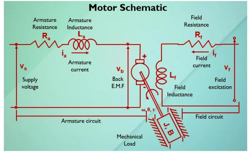
-> In motor mode, Vs is applied proggrassively, where Ia flows in armature circuit and residual magnetism in the field circuit will allow the rotor to start spinning.
-> When motor starts spinning, back emf (Vb) is generated and it opposes the supplied voltage.
-> Here, we supply voltage and once rotor starts spinning, it will drive a mechanical load with `w, theta and tau`.
-> Typically, Field excitation is set to a constant value, because we always need a magnetic field that constant.
-> Now, using Kirchoff's law, Vs is obtained, where Vb is directly propotional to `w` and T is directly propotional to Ia.
-> Then, Torque (T) is defined as the terms of J an B, where J = Moment of inertia of rotor and B = Viscous friction constant
-> Mathematically it can be represented as
`Vs = Ra*Ia+Vb+La*d(Ia)/dt`
`Vb = Kb*d theta/dt` and `T = Kt*Ia`
`T = B*w+J*(dw/dt)`
-> Simulink model is created as per the schematic diagram shown above. This model is solved for Vs in LHS.
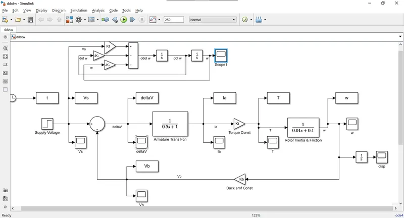
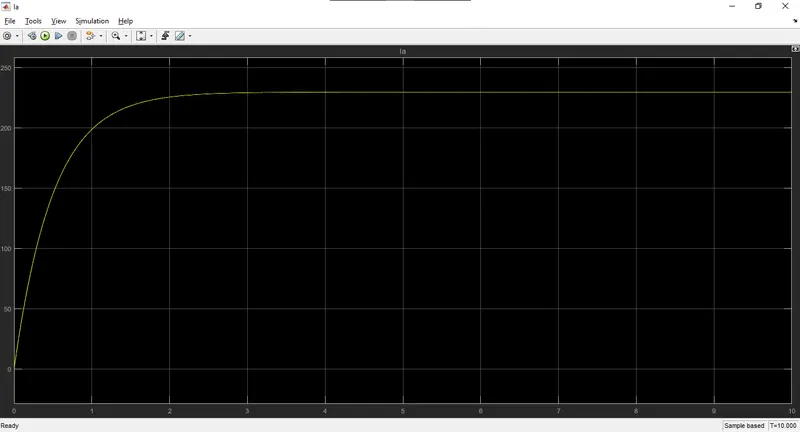
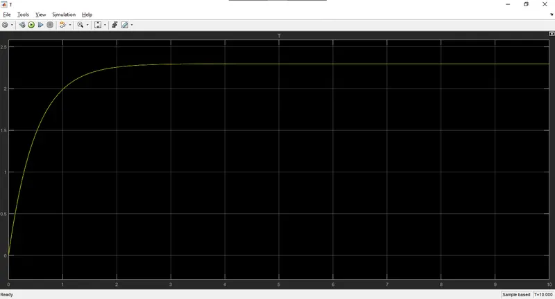
-> This is only basic Simulink model obtained for Vs and its two intermediate outputs are Ia, T and w.
-> The value of parameters considered are as shown below. Other parameter are also tried for the better output, but with this combination of parameter, we are getting the optimal signal output, which nearly critically damped. Other than this Vs = 230 V from t= 0 as a step i/p.
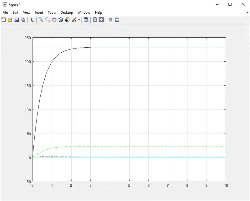
->The result gotten are shown as a Scope and Combined Plot below for the reference.
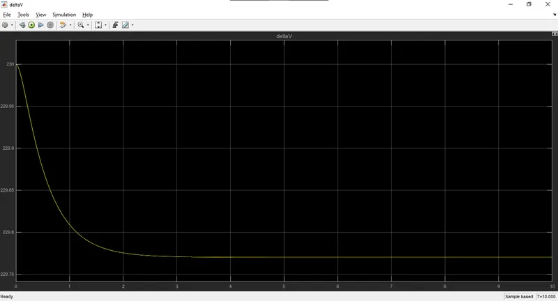
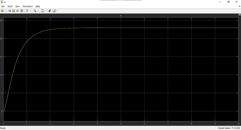
-> Speed of the rotor is regulated in between 20-25 rpm @ 230 V.
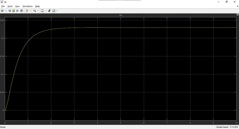
-> Apart from these, combined plot is shown below for reference purpose.
Use the Proportional, Integral, and Derivative (PID) control design knowledge gained in the training to design, develop and test a controller to maintain a desired speed for the motor.
Sol:
-> State-space model for the motor is shown in matrices form below.
-> `[[dw/dt], [di/dt]] = [[-B/J, (Kt)/J], [-(Kb)/(La), -(Ra)/(La)]]*[[dot theta], [dot i]] + [[0], [1/(La)]]*Vs`
-> `y = [[1] [0]]*[[dot theta], [dot i]] + [0]*Vs`
-> Tansfer Function is also as :
`(w(s))/(Vs(s)) = (Kt)/(J*La*s^2+(J*Ra+B*La)*s+(B*Ra+Kt*Km))`
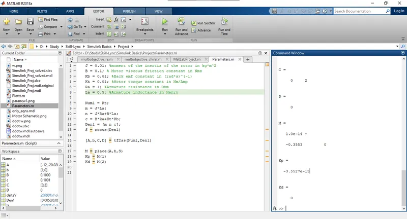
-> Now, Matrices A, B, C & D can be obtained directly from transfer function with the help of 'tf2ss'.
-> where, A is State matrix, B is Input matrix, C is Output matrix and D is Feedthrough matrix.
-> Now, from the obtained Numerator and Denominator, transfer function can be created and the poles also can be gotten from the function 'roots'.
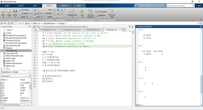
-> Now, to get Kp and Kd, matrices A & B and Poles also available. So function 'place' is used.
-> Syntax : K = place(A,B,P) ; where Kp = K(1) and Kd = K(2).
-> Ki is directly introduced in Simulink model via 'Gain' block.
-> These parameters, functions and its result are shown in MatLab below.
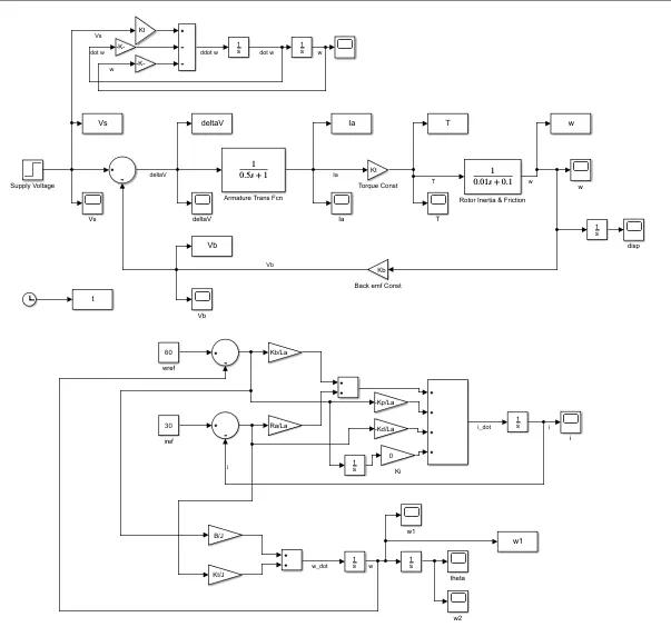
-> Now, from the transfer function, `ddotw = Kt*Vs-(J*Ra+B*La)*dotw-(B*Ra+Kt*Kb)w`. Simulink model is created within the basic model of DC motor. Model and its result scope block are shown below for reference.
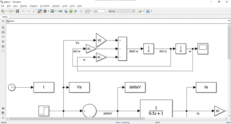
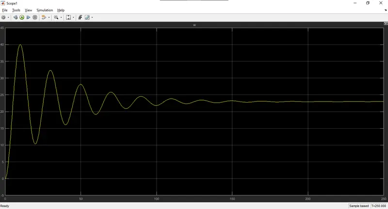
-> From the result, it can be said that output signal of w is evantually come to stable position, if we consider `ddot w` derived from transfer function.
-> Now, from the provided state-space model `[[dw/dt], [di/dt]] = [[-B/J, (Kt)/J], [-(Kb)/(La), -(Ra)/(La)]]*[[dot theta], [dot i]] + [[0], [1/(La)]]*Vs`, Simulink model can be created.
-> In this case, we can control `Ia` and `w` simultaneously. The Simulink model of this is shown below for reference.
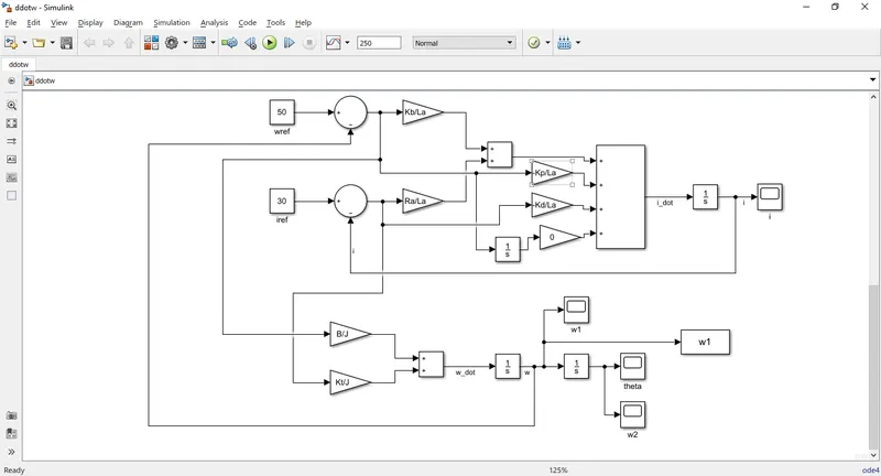
-> Here, wref is set to 50 and iref is set to 30.
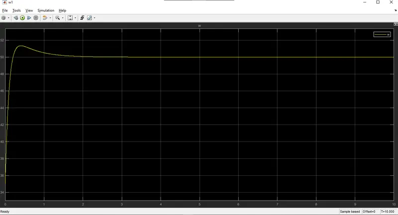
-> The result in the scope block of simulink is shown below for reference.
Case #1
Intial condition = 35.05, wref = 50
Case #2
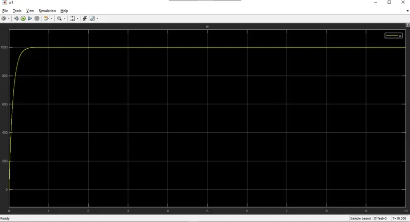
Initial condtion = 0, wref = 1000
Case #3
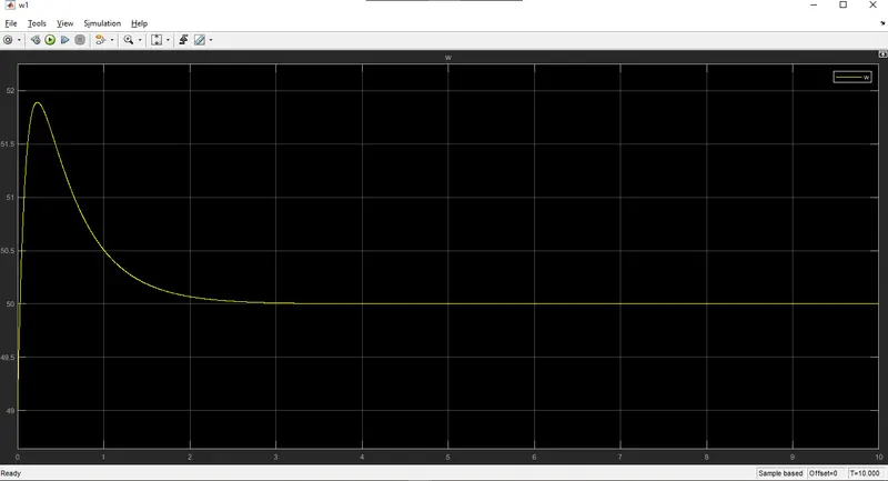
Initial condition = 49, wref = 50
Conclusion :
- In case 1 and 2, settling time < 2 sec, overshoot < 5% and Steady-state error <1%
- In case 3, setting time is nearly equal to 2 sec, overshoot is not in range, but can be controllable further and Steady-state errot <1%.
- Thus, objective of control design has been achived via this method.
- Controllable rpm of motor can be achieved at any initial condition and any reference point. So we can consider it as a govering method to regulate 'w'.
- The concluding simulink model is shown below.