Project - Speed Control of a Direct Current (DC) motor
Aim: To build a Simulink model for the DC machine by following the mathematical representation, to design a PID controller to attain a desirable speed.
Theory: DC motors have speed control capability, which means that speed, Torque, and even direction of the rotor can be changed at any time to meet new conditions.
The motor torque T, is related to the armature current ia, by a constant factor Kt.
`T = Kt * ia`
for getting the desirable speed I am going to change the armature current and gradually the change of speed is attained.
from Newton's law combined with Kirchoff's law
`Jxxddottheta + B xx dottheta = Ktxx Kmxxia`
`Lxx(dia)/dt + Ra xxia = Vs-KtKmxxdottheta`
using Laplace transforms the above modeling equations can be expressed in terms of s for open loop transfer function
`(omega(S))/(Vs(S))= (Kt)/((La*S+Ra)(J*S+b)+KtKm)`
where `1/(La*S + Ra)` represents armature
`1/(J*S+b)` represents rotor inertia and friction
DC Motor: By considering the above-mentioned equations the following parameters are considered and programmed in Matlab and saved in a file named dc_machine_parammeters.m and attached.
%This file contains design parameters to model DC motor
J = 0.01; % moment of inertia of the rotor in kg-m^2
b = 0.1; % motor viscous friction constant in N-m-s
Km = 0.01; % Back EMF Constant in v/rad/s
Kt = 0.01; % Motor torque constant in N-m/amp
Ra = 1.0; % resistance of armature circuit in ohms
La = 0.5; % Inductance of the armature circuit in henries
by these parameters, the DC motor model is built
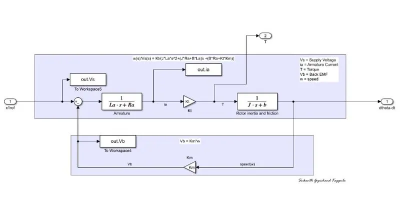
the open loop transfer function is fed back with a back EMF
`Vb = Km xx dottheta`
PID controller:
PID controllers are commonly used to regulate the time-domain behavior of many different types of dynamic systems.
I am considering the feedback system architecture where the DC motor is the plant where the speed of the DC motor must be accurately regulated to attain a desirable speed.
the PID controller can be represented as
`u(t) = kp xx e(t) + kixxinte(tau) xx d tau -kd xx (de(t))/dt`
the PID controller is placed in the forward path so that its output becomes the voltage applies to the motor's armature.
the output signal y(t) is `(d theta)/dt which refers to the speed `omega`
the designed DC motor representation is fitted in the subsystem to clearly understand the control system.
By pole placement method the Kp and Kd is defined
for that, the state space model of the DC motor is concluded
`d/dt[(theta), (i)] =[[-b/J,(Kt)/J],[(-Km)/La,(-Ra)/(La)]][(theta),(i)] + [(0),(1/(La))]Vs`
`y(t) = [[1,0]][(theta),(i)]`
these state space models are calculated as follows
zeta = 0.8;
wn = 2*pi;
p1 = -zeta*wn+wn*sqrt(zeta^2-1);
p2 = -zeta*wn-wn*sqrt(zeta^2-1);
P = [p1;p2];
A = [-b/J Kt/J;-Km/La -Ra/La];
B = [0;1/La];
By the above values, the pole placement method is used
K = place(A,B,P);
Kp = [K(1,1)];
Kd = [K(1,2)];
Ki = 40;
now the built model is
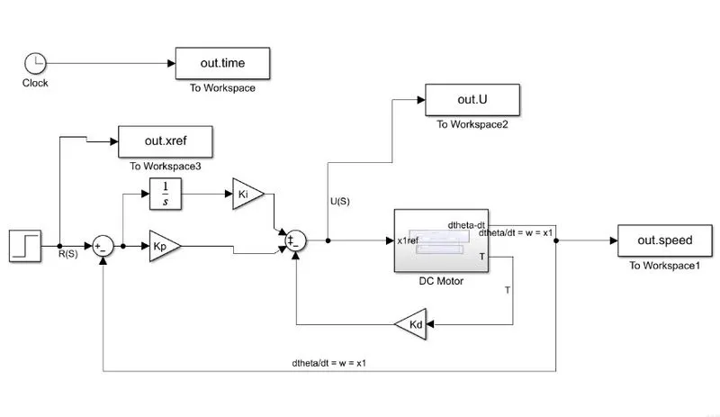
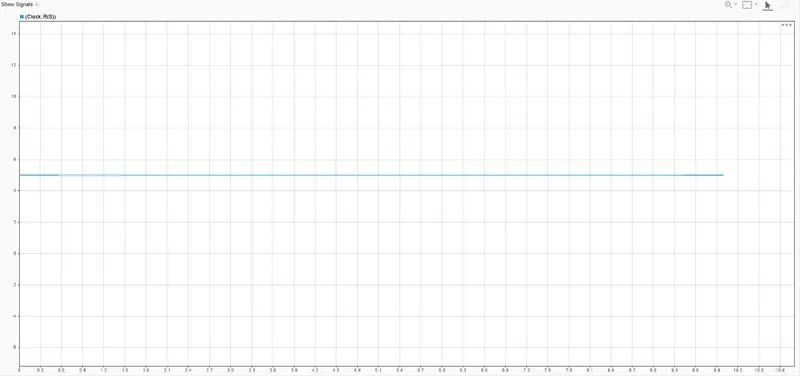
the input is considered to be step with step time 0 and final time is 5
now the input signal is
the values of zeta and Ki(integral gain) are decided by trial and error method
the best value for zeta for a suitable curve for speed is around 0.99
Matlab does not allow the zeta value 1 to show pole place error
i go with zeta = 0.99 which is a better response
for Ki, I have gone through many iterations in which
Ki = 10 steady-state error and setting time are poor
ki = 20 the same
ki = 30 setting time is a little bit poor but if Matlab allows us for zeta = 1 the setting time is <2s
ki = 40 overshoot is poor
gradually the overshoot is raising as Ki value increases
so, fixing to the value of Ki = 30
Output:
the following program lets us to plot the speed, control signal curves
figure(1);
plot(out.time,out.speed,'m--');
grid;
title('speed');
figure(2);
plot(out.time,out.U,'m--');grid;hold;
plot(out.time,out.xref,'b-');
title('U(S) & R(S)');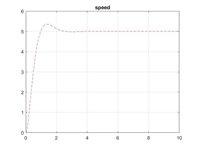
and the control signal and reference signal are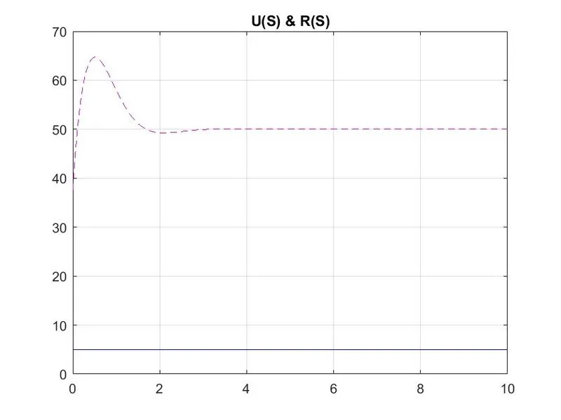
now we can observe a better corve that the setting time if Matlab allows us for zeta to be 1 then the setting time is <2s
overshoot<5%
steady-state error <1%
the plots are plotted by the following program
the desired speed is attained by the PID Controller
the above procedure is achieved by pole placement method where Kp, Kd is achieved by place command
we can achieve a better-sustained curve by trail and error method where Kp, Kd and Ki are achieved by itterations in which i got Kp=50, Kd=10 and Ki = 100
which sattisfies the control design objectives.
Conclusion: From the above simulation I know that kp will have the effect of reducing the rise time; ki will have the effect of eliminating the steady state error, kd will have the effect of increasing the stability of the system, reducing the overshoot and improving the transient response. Thus the desired speed of a DC motor is attained by the designed and developed PID controller for DC motor first principles is simulated.