Project - Speed Control of a Direct Current (DC) motor

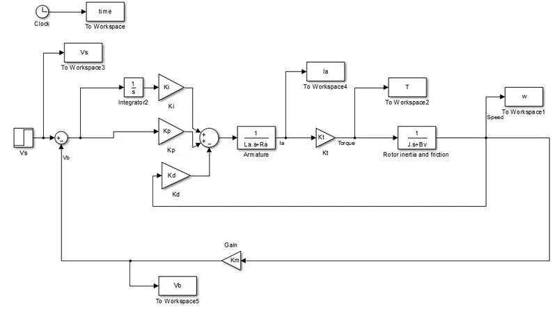
A simulink model of the DC motor is developed as in the schematic and the PID controller is designed

%Design parameters to deisgn DC motor
J = 0.01; %Moment of inertia in kg-m^2
Bv = 0.1; %Motor viscous friction in N-m-s
Km = 0.01; % Back emf constant in volts/rad/sec
Kt = 0.01; % Motor torque constant in N-m/amp
Ra = 1; %Resistance of armature in ohm
La = 0.5; %Inductance of armature in henry

zeta = 1.001; %slightly critically system
fn = 1.0; % Design parameters
wn = 6.28;
p1 = -zeta*wn+wn*sqrt(zeta^2-1); %Desired poles
p2 = -zeta*wn-wn*sqrt(zeta^2-1);
P = [p1;p2];
A = [-Bv/J Kt/J;-Km/La -Ra/La];
B = [0;1/La];
K = place(A,B,P);

The pole placement design gains are used as starting values for Kp and Kd gains for the PID design setting Ki to zero initially. i.e (Kp = 6.8464, Kd = 0.2863 and Ki = 0)

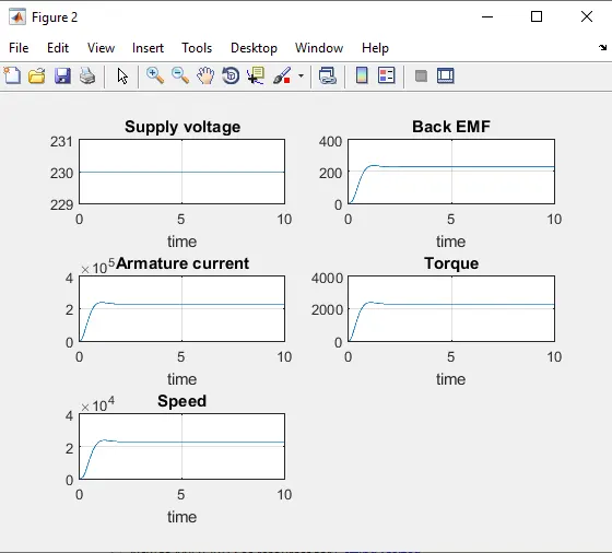
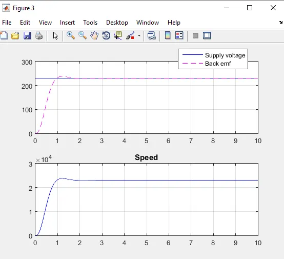
A new set of gain values are obtained after tuning the controller. The proportional gain did not affect much on the response but the integral gain helped in reducing the steady state error as well as the settling time and the derivative gain helped in reducing the overshoot. The plot after taking the new set of gain values is plotted and hence the desired speed of the motor is achieved.

%New feedback gains that fulfill the requirement of Settling time <2seconds,Overshoot < 5%, Steady state error < 1%

Kp = 6.8464;
Kd = 18;
Ki = 6000;

Response when Kp, Kd values are taken from the gain matrix K and Ki is set to zero

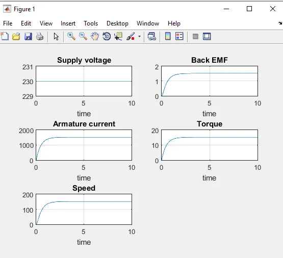
Figure 2 and Figure 3 shows the Response after tuning the PID controller and the corresponding values obtained for Kp, Ki and Kd are