Challenge

Project - Speed Control of a Direct Current (DC) motor

AAsif Ahmed24 Aug 2022

Project

In this project, a Simulink model for the DC motor will be first developed per the schematic shown in Figure 1.

Use the Proportional, Integral, and Derivative (PID) control design knowledge gained in the training to design, develop and test a controller to maintain a desired speed for the motor.

Answer:

PID Control of a DC Motor

DC Machine:

A DC machine functions as a generator or motor.

Rotor with an armature winding providing the electric circuited.

Stator with field winding serving as a magnet when energized.

A prime mover is coupled with the rotor, allowing it to rotate in the magnetic field created by the
field winding.

This mechanism induces EMF in the conductors mounted on the rotor contribute to voltage
generation.

The electrical energy supplied to armature winding and the field winding contributes to a rotating
magnetic field that forces the rotor to rotate.

Motor Schematic Diagram

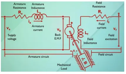
Using Krichhoff’s Voltage law, one can derive,

vs = Raia + La (dia/dt)+ Vb

Vs = Supply Voltage
Ra = Armature Resistance
Ia = Armature Current
La = Armature Inductance
Vb = Back EMF

Back EMF, angular velocity and torque are related by,

vb = Km (dθ/dt) τ = Kti

Here, Km and Kt are the back EMF and torque constants respectively,

Angular Velocity,

ω = θ dot

The open loop transfer function for the motor with the speed (w) and supply voltage (Vs) can be derived
as,

PID – Design for speed control of a DC motor:

Build a Simulink model of PID controller to regulate the speed of the DC Motor.

We will assume that the input of the system is the voltage source (V) applied to the motor's armature, while the output is the rotational speed of the shaft.

Hence for that we have to assume below few parameters to build a PID Controller.

Moment of inertia of the rotor (J) = 0.01 kg.m^2

Motor viscous friction constant (b) = 0.1 N.m.s

Electromotive force constant (Km) = 0.01 V/rad/sec

Motor torque constant (Kt) = 0.01 N.m/Amp

Armature resistance (Ra) = 1 Ohm

Armature inductance (La) = 0.5 H

The torque generated by a DC motor is proportional to the armature current and the strength of the magnetic field.

Steps to be followed in MATLAB software.

1. Click on MATLAB software.

2. Click on Simulink in MATLAB Software.

3. Click on Library.

4. Drag the blocks which are used to build a PID controller.

5. After dragging the blocks give names to the respective block.

6. Connect the blocks to each other to find the solution.

7. Set the timing in the simulink command.

7. Save the file

8. Run the simulation.

Step function is used with supply voltage of 230v.

In MATLAB writing below program in editor command.

% Design Parameters

J=0.01;

B=0.1;

Km=0.01;

Kt=0.01;

Ra=1.0;

La=0.5;

% Nomial parameters of the spring mass system

m=100.0;

k=3944.0;

% Equivalent wn

wn=6.2832; % sqrt(k/m) rad/s

fn=1.0; % wn/(2*pi) Hz

% Design parameters

zeta=0.5; % Under damped system

% Desired poles

p1=-zeta*wn+wn*sqrt(zeta^2-1);

p2=-zeta*wn-wn*sqrt(zeta^2-1);

P=[p1;p2];

% A & B matrices

A=[0 1;-k/m 0];

B=[0;1/m];

% Pole placement design

K=place(A,B,P);

% Kp and Kd are obtained from an earlier design using the PLACE commond

Kp=3.86;

Kd=628.32;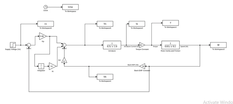

% Design Parameters
J=0.01;
B=0.1;
Km=0.01;
Kt=0.01;
Ra=1.0;
La=0.5;

% Nomial parameters of the spring mass system
m=100.0;
k=3944.0;

% Equivalent wn
wn=6.2832; % sqrt(k/m) rad/s
fn=1.0; % wn/(2*pi) Hz

% Design parameters
zeta=0.5; % Under damped system

% Desired poles
p1=-zeta*wn+wn*sqrt(zeta^2-1);
p2=-zeta*wn-wn*sqrt(zeta^2-1);
P=[p1;p2];

% A & B matrices
A=[0 1;-k/m 0];
B=[0;1/m];

% Pole placement design
K=place(A,B,P);

% Kp and Kd are obtained from an earlier design using the PLACE commond
Kp=3.86;
Kd=628.32;

Simulink Block Diagram for PID with DC Motor

Plots are obtained by writing below program in Matlab Window.

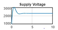
subplot(321);plot(time,Vs);grid;
subplot(321);title('Supply Voltage');
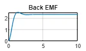
subplot(322);plot(time,Vb);grid;
subplot(322);title('Back EMF');
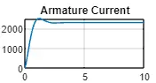
subplot(323);plot(time,Ia);grid;
subplot(323);title('Armature Current');
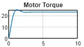
subplot(324);plot(time,T);grid;
subplot(324);title('Motor Torque');
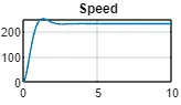
subplot(325);plot(time,W);grid;
subplot(325);title('Speed');
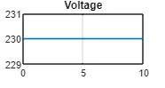
subplot(326);plot(time,cs);grid;
subplot(326);title('Voltage');

subplot(321);plot(time,Vs);grid;
subplot(321);title('Supply Voltage');
subplot(322);plot(time,Vb);grid;
subplot(322);title('Back EMF');
subplot(323);plot(time,Ia);grid;
subplot(323);title('Armature Current');
subplot(324);plot(time,T);grid;
subplot(324);title('Motor Torque');
subplot(325);plot(time,W);grid;
subplot(325);title('Speed');
subplot(326);plot(time,cs);grid;
subplot(326);title('Voltage');

Hence below plots are obtained.