Project 2
Project 2
Description:
As discussed in Lecture 11, Project 2 deals with the development of a forward energy-based fuel consumption model of a P1 hybrid vehicle. This model is based on the conventional vehicle model from Project 1.
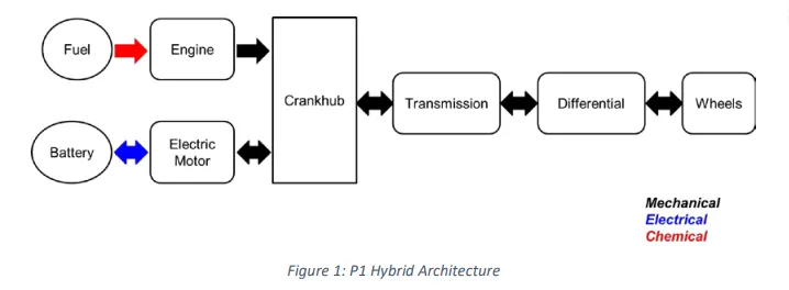
The main goal of this project is to understand the functionality of a P1 hybrid and be able to model it.
Honda Insight motor and battery are considered for this project. Data is taken from ADVISOR data base developed by NREL, USA. Data provided in the project files.

“Project2_InitFile.m” is a Matlab script used to load all the variables required for running the Simulink model and for post-processing. The drive cycle selection is also done here. Before running the Simulink vehicle model, run this initialization script.
Task:
The task of this project is to quantify the improvement in fuel economy numbers for the hybrid vehicle (kmpl), compared to the conventional vehicle, on the urban cycle (UDDS) and highway cycle (HWFET). Also, to analyze and understand the vehicle operating points in terms of engine and motor speed, torque, transmission speeds, pedal positions, gear, distance traveled, battery voltage, current, SoC etc.
To do that, the following steps need to be followed:
1) Load the Project2 folder as the Current Folder in Matlab.
2) Run the “Project2_InitFile.m” Matlab script.
3) Copy the Conventional vehicle Simulink model created for Project 1 in this folder. Figure 1: P1 Hybrid ArchitectureHybrid Drives Development
4) Modify this model into a hybrid vehicle model. The lecture presentations can be used as reference. Battery and Supervisory controller models developed in the assignments can be reused.
5) Add additional ‘To Workspace’ blocks for transferring the desired Simulink vehicle data into the Matlab workspace.
6) Simulate the hybrid model on the desired drive cycles.
7) Write a project report that contains the following:
a. Tabulate the fuel economy numbers (kmpl) for UDDS and HWFET cycle. Compare these numbers with the baseline numbers for conventional vehicle model from Project 1.
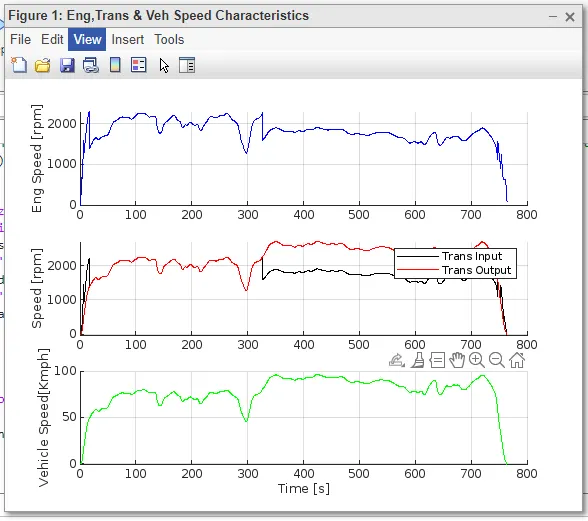
b. Plot the time trace for engine, transmission input, transmission output and wheel speed on one plot.
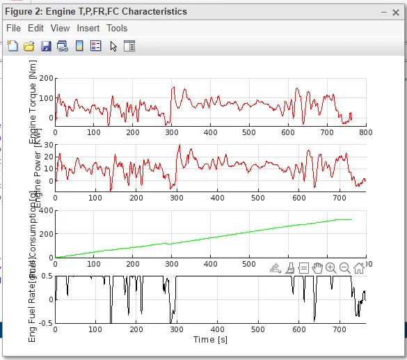
c. Plot engine torque, engine power, fuel rate and fuel consumption using subplots.
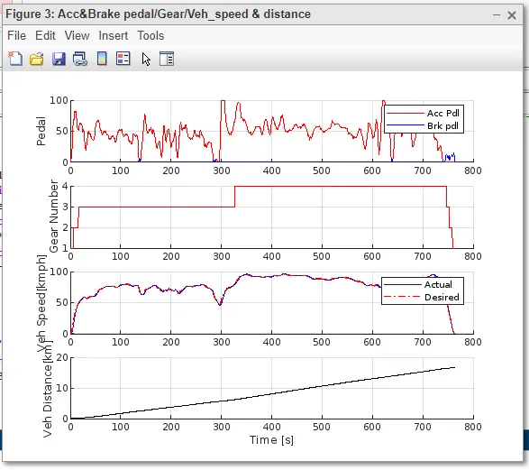
d. Plot accelerator and brake pedal, gear command, vehicle desired and actual speed, vehicle distance using subplots.
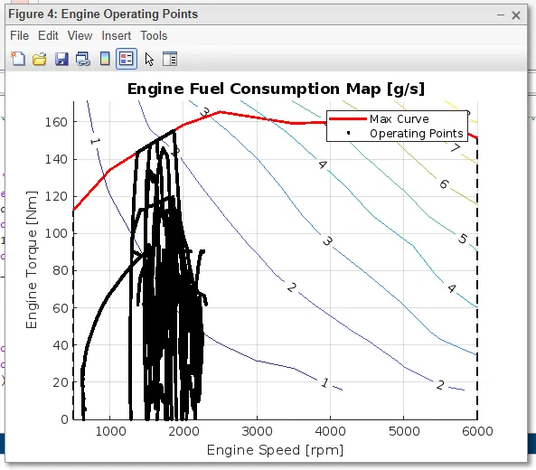
e. Plot the engine operating points on the engine fuel map.
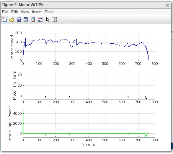
f. Plot motor speed, torque, motor input power using subplots.
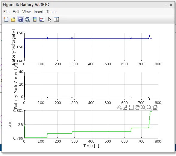
g. Plot pack voltage, current and SoC using subplots.
h. Plot the motor operating points on the motor input power map, with the motor max motoring and generating torque curves.
i. Write down appropriate brief comments on each of these plots, describing the vehicle behavior throughout the drive cycle.
j. Generate the plots for both drive cycles
Solution:
Forward-Modelling Approach
The forward modelling approach is also known as cause-effect, engine-to-wheel or rear-to-front method. The direction of calculation is the same as the direction of positive power flow, from engine-to-wheel.
This approach is based on vehicle dynamics equations and the behaviour of each powertrain components and their dynamic interaction.
Moreover, a driver controller is required to control the vehicle to follow a desired speed and set the start of the
calculations. The controller is implemented to model the driver that will either push the accelerator or the brake
pedal to match the desired speed which enables to study the driver behaviour. The controller is used as part of
a feedback loop that will determine the energy required to drive the vehicle.
P1 Hybrid
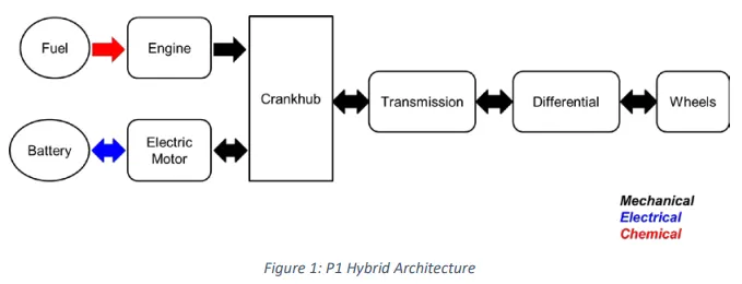
Honda Insight motor and battery are considered for this project. Data is taken from ADVISOR data base
developed by NREL, USA. Data provided in the project files.

VEHICLE MODEL
Initial File
A MATLAB script has been created to load all the variables needed to run and post-process the Simulink model.
Drive cycle selection is also done from here. Before running the Simulink vehicle model, the script is initialized at MATLAB to load all the variables in the workspace.
Following program is loaded in Script Window.
%%%%%%%%%%%%%%%%%%%%%%%%%%%%%%%%%%%%%%%%%%%%%%%%%%%%%%%%%%%%%%%%%%%%%
%% Skill-Lync -> Hybrid Drives Development
% Project 2 - Conventional Vehicle Model
% By - Ullekh Gambhira

% Description:

%% Initialization File
% Initialization file for loading the variables for the Conventional vehicle simulation model

%% Vehicle Parameters
clc
clear all
M = 1500;       % Vehicle weight [kg]
Cr = 0.015;     % Rolling resistance coefficient
Rw = 0.35;      % Rolling radius [m]
Cd = 0.33;      % Drag coefficient
Af = 2;         % Frontal area [m2]
rhoa = 1.225;   % Air density [kg/m3]
Vwind = 0;      % Wind velocity [kmph]
g = 9.81;       % Gravitational acceleration [m/s2]
theta = 0;      % Slope [deg]
myu_road_tire = 1; % Coefficient of friction between tire - road interface

%% Powertrain Parameters
FDR = 3.73;                         % Final Drive Ratio / Diff Ratio
DiffEff = 0.99;                     % Differential efficiency (assumed independent of operating conditions)

NumGear = 4;                        % Number of gears in transmission
TransGear = [1:NumGear];            % Transmission Gears
TransRatio = [3.06, 1.62, 1, 0.7];  % Corresponding Transmission ratios
TransEff = 0.90;                    % Transmission efficiency (assumed independent of operating conditions)

TC_SR = [0, .5, .6, .7, .8, .87, .92, .94, .96, .97, 1];   % Torque Converter Speed Ratio (Matlab default) -> TurbSpd/PumpSpd
TC_TR = [2.232, 1.5462, 1.4058, 1.2746, 1.1528, 1.0732, 1.0192, 1, 1, 1, 1];   % Torque Converter Torque Ratio (Matlab default) -> TurbTrq/PumpTrq
TC_Cf = 1e-4 * [.72558, .66322, .63463, .59042, .51331, .4144, .29287, .22444, .12186, .04386, 0]; % Torque Converter Capacity Factor (Matlab default) -> PumpTrq/PumpSpd^2 [Nm/rpm^2]

load Engine_data_1_9L_Saturn_95kW
load Trans_Shift_map
load EM_Honda_Insight_10kW
load ESS_NiMH6


ESS_init_soc = 0.8;
ESS_soc_max = 0.9;
ESS_soc_min = 0.6;


%% Driver Parameters
Kp = 10;                    % P gain for driver PI model
Ki = 1;                     % I gain for driver PI model
Drive_Cycle_Select = 2;     % Drive cycle selection

% Drive cycle values in m/s

if Drive_Cycle_Select == 1
    load UDDS;

elseif Drive_Cycle_Select == 2
    load HWFET;

elseif Drive_Cycle_Select == 3
    load FTP;

elseif Drive_Cycle_Select == 4
    load US06;

elseif Drive_Cycle_Select == 5
    load NEDC;

elseif Drive_Cycle_Select == 6
    load WLTP;

end

time_end = cyc_time(end);
vel_end = cyc_vel(end);
%%%%%%%%%%%%%%%%%%%%%%%%%%%%%%%%%%%%%%%%%%%%%%%%%%%%%%%%%%%%%%%%%%%%%
%% Skill-Lync -> Hybrid Drives Development
% Project 2 - Conventional Vehicle Model
% By - Ullekh Gambhira
% Description:
%% Initialization File
% Initialization file for loading the variables for the Conventional vehicle simulation model
%% Vehicle Parameters
clc
clear all
M = 1500; % Vehicle weight [kg]
Cr = 0.015; % Rolling resistance coefficient
Rw = 0.35; % Rolling radius [m]
Cd = 0.33; % Drag coefficient
Af = 2; % Frontal area [m2]
rhoa = 1.225; % Air density [kg/m3]
Vwind = 0; % Wind velocity [kmph]
g = 9.81; % Gravitational acceleration [m/s2]
theta = 0; % Slope [deg]
myu_road_tire = 1; % Coefficient of friction between tire - road interface
%% Powertrain Parameters
FDR = 3.73; % Final Drive Ratio / Diff Ratio
DiffEff = 0.99; % Differential efficiency (assumed independent of operating conditions)
NumGear = 4; % Number of gears in transmission
TransGear = [1:NumGear]; % Transmission Gears
TransRatio = [3.06, 1.62, 1, 0.7]; % Corresponding Transmission ratios
TransEff = 0.90; % Transmission efficiency (assumed independent of operating conditions)
TC_SR = [0, .5, .6, .7, .8, .87, .92, .94, .96, .97, 1]; % Torque Converter Speed Ratio (Matlab default) -> TurbSpd/PumpSpd
TC_TR = [2.232, 1.5462, 1.4058, 1.2746, 1.1528, 1.0732, 1.0192, 1, 1, 1, 1]; % Torque Converter Torque Ratio (Matlab default) -> TurbTrq/PumpTrq
TC_Cf = 1e-4 * [.72558, .66322, .63463, .59042, .51331, .4144, .29287, .22444, .12186, .04386, 0]; % Torque Converter Capacity Factor (Matlab default) -> PumpTrq/PumpSpd^2 [Nm/rpm^2]
load Engine_data_1_9L_Saturn_95kW
load Trans_Shift_map
load EM_Honda_Insight_10kW
load ESS_NiMH6
ESS_init_soc = 0.8;
ESS_soc_max = 0.9;
ESS_soc_min = 0.6;
%% Driver Parameters
Kp = 10; % P gain for driver PI model
Ki = 1; % I gain for driver PI model
Drive_Cycle_Select = 2; % Drive cycle selection
% Drive cycle values in m/s
if Drive_Cycle_Select == 1
load UDDS;
elseif Drive_Cycle_Select == 2
load HWFET;
elseif Drive_Cycle_Select == 3
load FTP;
elseif Drive_Cycle_Select == 4
load US06;
elseif Drive_Cycle_Select == 5
load NEDC;
elseif Drive_Cycle_Select == 6
load WLTP;
end
time_end = cyc_time(end);
vel_end = cyc_vel(end);
Simulink Model
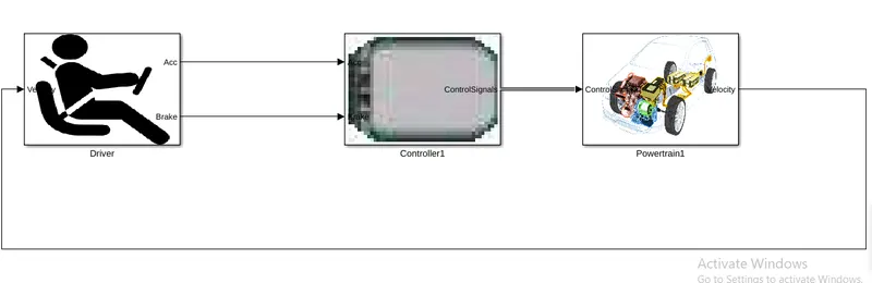
As shown in above model, 3 models are connected to each other
Driver - Controller - Powertrain
The actual vehicle speed is given as feedback to the driver block, and the driver block gives the controller block the required acceleration or brake output, while the controller block provides control signals for engine torque, gear shifting and brake torque to the Powertrain model.
Driver Model
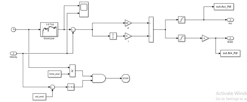
Driver Model is a basic PI controller that generates accelerator and brake pedal outputs to match the desired and actual vehicle speeds.
The PI controller controls the error between the required drive cycle and actual vehicle speed by providing acceleration and brake pedal output to the controller.
Controller Model
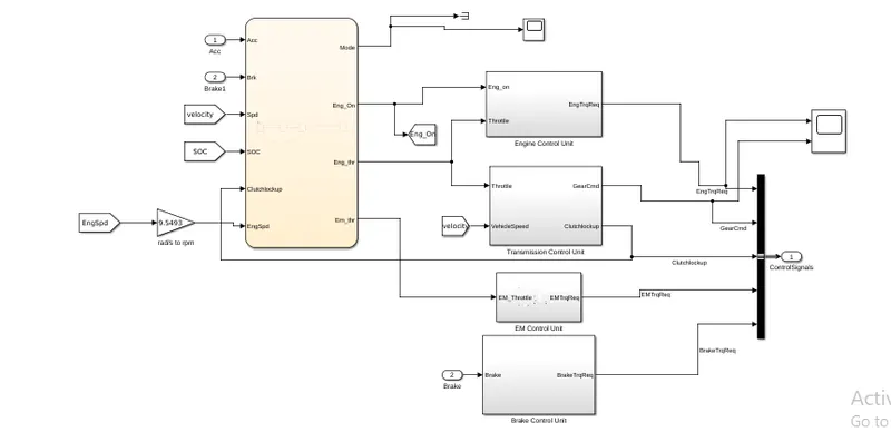
The 'Controller block is the brains of the vehicle, representing the electronic controls units. Based on the driver
inputs, it generates desired engine torque, desired motor torque, desired transmission gear and desired brake
torque. These inputs are fed to the 'Powertrain' block which represents the drivetrain of the vehicle
A state flow machine is used to represent the supervisory control unit, which decides the operationg mode.
while it is start/stop mode or cruising mode or regen braking mode. for each modes the Engine drive and the
motor drive are controlled.
State Flow Chart
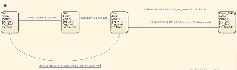
The Input to the state flow charts is Acceleration and Brake pedal input from the driver unit, Engine actual
speed, Actual vehicle speed, SOC status and the clutch lockup state. And the State flow Outputs to the
individual controllers are the Mode, Engine On/ off request, Engine input throttle and Electric motor input Throttle
The controller consists of an engine control unit, a transmission control unit, Electric Motor control unit and a
brake control unit.
All control signals re passed to transmission model which represents the drive train.
Engine Control Unit Model
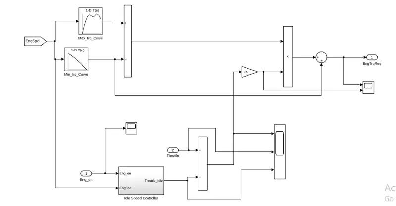
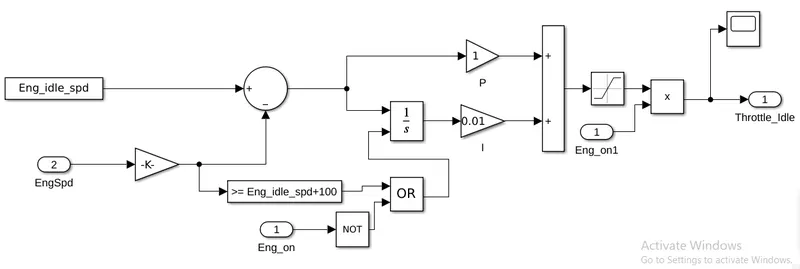
Idle Speed Controller Model
Transmissin Control Unit Model
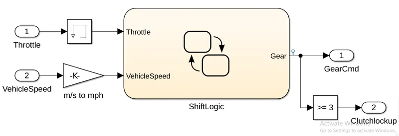
Shift Logic Model
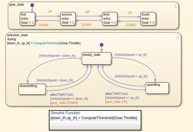
The Gear shifting is Controlled according to the vehicle speed and throttle input.
The gear command is passed to the Transmission block to select the desired gear ratio.
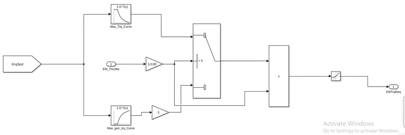
EM Control Unit Model
Brake Control Unit Model
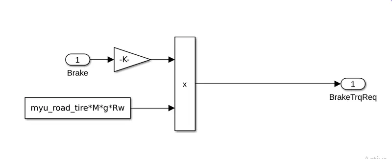
Brake Control unit Produce required brake torque according to the brake pedal input and passes the brake torque in to the wheel block in the transmission model.
Power Train Model
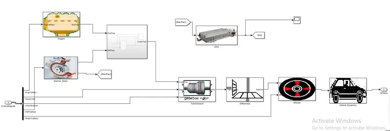
The powertrain model includes all the components that convert the power of the engine into vehicle motion.
This includes Engine, Battery Pack, Electric Motor, Crank Hub, Transmission, Differential, Wheels and the vehicle
body dynamics subsystems.
The control signals from the control model are transmitted via a bus to the corresponding blocks in the
powertrain model.
Engine Model
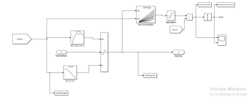
Based on the Engine speed The required torque from the controller is saturated between Max torque curve and min torque curve and passes the Engine torque to the Transmission block.
The 2D lookup table is used to calculate the fuel flow rate based on engine speed and engine torque. The fuel flow rate is then integrated to find the fuel consumption.
Estimated fuel flow rate, fuel consumption, engine torque and engine speed are passed to the MATLAB workspace using the to-workspace block.
Engine fuel flow rate and Fuel consumption are scoped.
Electric Motor Model
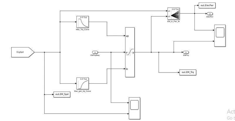
Based on the Engine speed The required EM torque from the controller is saturated between Max EM torque
curve and max EM torque Generation curve and passes the EM torque to the Crank Hub.
The 2D lookup table is used to calculate the Input Electric Power to the Motor based on EM speed and EM torque.
Crankhub Model
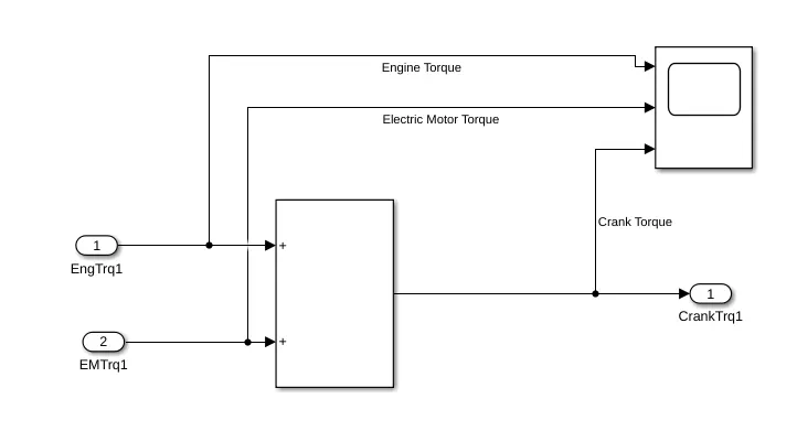
Transmission Model
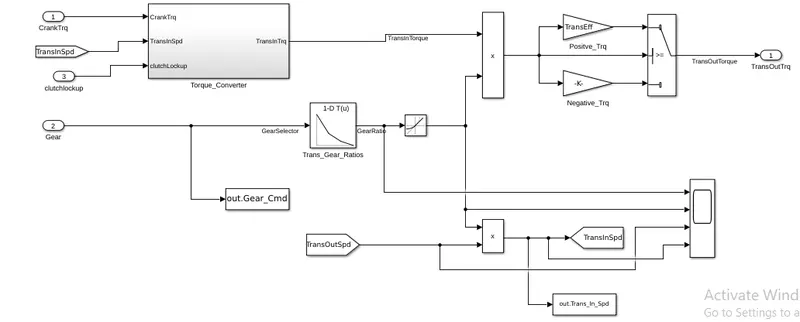
The Crank is connected to the automatic transmission via a torque converter. The output of the transmission is
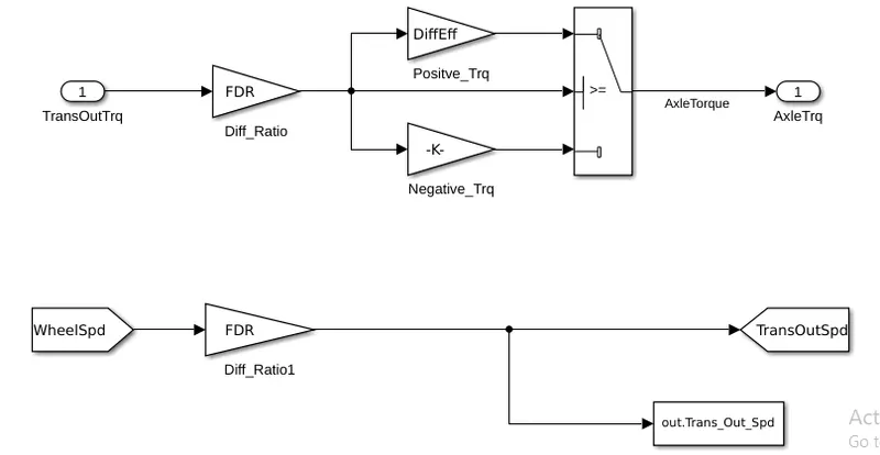
connected to the differential.
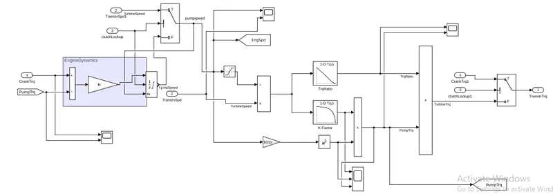
New Clutch LockUp feature is adding to this Hybrid version.
Torque Converter Model
Differential Model
Wheel Model
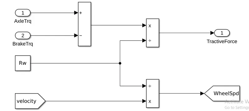
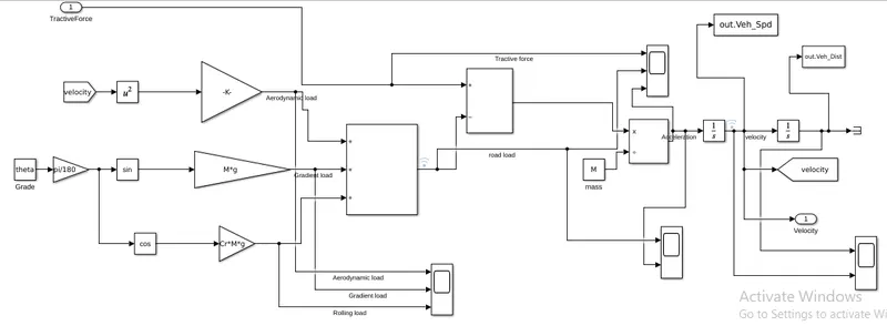
Vehicle Dynamic Model
ESS Model
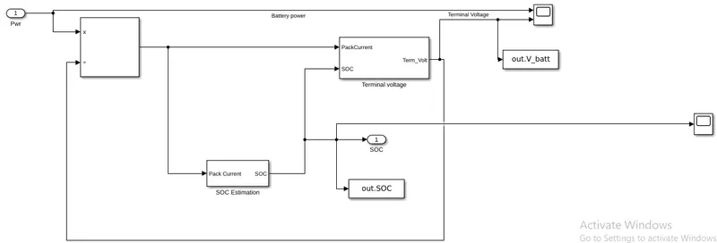
A Battery pack Subsystem is created with Electric power input, and Battery SOC as output.
2 different subblocks have been created to determine the SOC and terminal voltage separately, the SOC being
used to calculate the terminal voltage.
Terminal Voltage Model
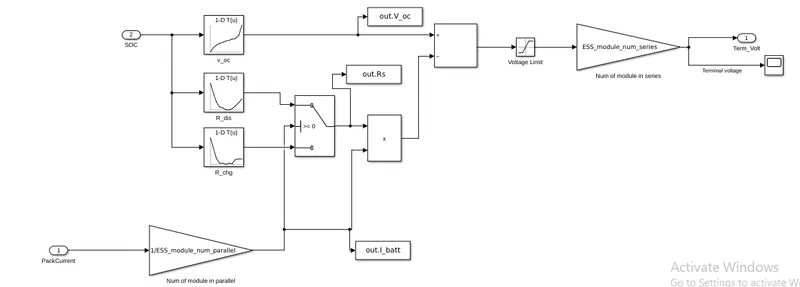
Ideal voltage and internal resistance are determined by ID lookup tables, and battery voltage is determined
using the model.
The specified values are sent back to workspace using the Two Workspace block and can used for post
processing.
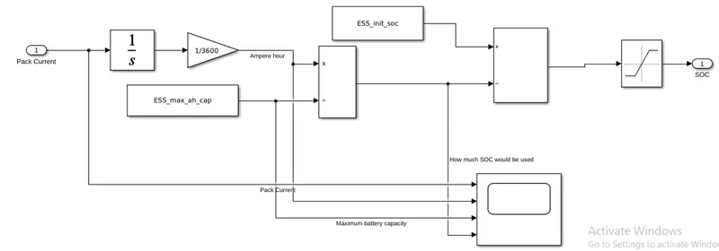
SOC Estimation Model
Processing File
Following program is written in Script Window to get results
%%%%%%%%%%%%%%%%%%%%%%%%%%%%%%%%%%%%%%%%%%%%%%%%%%%%%%%%%%%%%%%%%%%%%
%% Skill-Lync -> Hybrid Drives Development
% Project 2 - Hybrid Electric Vehicle Model
% By - Ullekh Gambhira

% Description:
% The following file is to used with the Initialization file and Simulink
% results for post-processing of the data.
% The file is incomplete, has some examples of how the data is imported
% into a readable format, data analysis and plotting examples.
% Based on the project task, use commands in a similar format as given
% below, to analyse the data and generate required plots.
% You can change variable names if desired

%% Post-Processing File
%  File for post-processing the Conventional vehicle simulation model data

%% Renaming variables
Time = out.tout;
Acc_Pdl = out.Acc_Pdl;          % Accelerator pedal [%]
Brk_Pdl = out.Brk_Pdl;          % Brake pedal [%]
Gear_Cmd = out.Gear_Cmd;        % Transmission gear
Trans_In_Spd = out.Trans_In_Spd*30/pi;  % Transmission input speed [rpm]
Trans_Out_Spd = out.Trans_Out_Spd*30/pi;% Transmission output speed [rpm]
Eng_Trq = out.Eng_Trq;          % Engine brake torque [Nm]
Eng_Spd = out.Eng_Spd*30/pi;    % Engine speed [rpm]
Eng_Fuel_Consump = out.Eng_Fuel_Consumption;    % Engine fuel consumption [g]
Veh_Dist = out.Veh_Dist/1000;     % Distance traveled by vehicle [km]
Veh_Spd = out.Veh_Spd.*18/5;      % Vehicle speed [kmph]
Eng_Fuel_Rate=out.Eng_Fuel_Rate;  % Engine fuel rate [gm/sec]
Veh_Desired_Speed = out.Veh_Desired_Speed.*18/5 ; %Desired vehicle speed [kmph]

%% Data Analysis
Eng_Pwr = Eng_Spd.*pi/30.*Eng_Trq/1000;   % Engine brake power [kW]
rho_petrol = 0.7197;                    % Density of petrol [kg/L]
kmpl = Veh_Dist(end)/(Eng_Fuel_Consump(end)/1000/rho_petrol);    % Fuel economy [kmpl]


%% Plotting vehicle characteristics time trace

% a. Tabulate the fuel economy numbers (kmpl) for UDDS and HWFET cycle.
Fuel_Economy = kmpl

%% b. Plot the time trace for engine, transmission input, transmission output and wheel speed on one plot.

figure('Name','Eng,Trans & Veh Speed Characteristics')

subplot(3,1,1)
hold on
grid on
plot(Time, Eng_Spd, 'linewidth', 1, 'Color', 'blue');
ylabel('Eng Speed [rpm]')

subplot(3,1,2)
hold on
grid on
plot(Time, Trans_In_Spd, 'linewidth', 1, 'Color', 'black');
plot(Time, Trans_Out_Spd, 'linewidth', 1, 'Color', 'red');
ylabel('Speed [rpm]')
legend('Trans Input','Trans Output');

subplot(3,1,3)
hold on
grid on
plot(Time, Veh_Spd, 'linewidth', 1, 'Color', 'green');
xlabel('Time [s]');
ylabel('Vehicle Speed[Kmph]');

% c. Plot engine torque, engine power, fuel rate and fuel consumption using subplots.
figure('Name','Engine T,P,FR,FC Characteristics')

subplot(4,1,1)
hold on
grid on
plot(Time, Eng_Trq, 'linewidth', 1, 'Color', 'red');
ylabel('Engine Torque [Nm]')

subplot(4,1,2)
hold on
grid on
plot(Time, Eng_Pwr, 'linewidth', 1, 'Color', 'red');
ylabel('Engine Power [KW]')
xlim([0, Time(end)]);

subplot(4,1,3)
hold on
grid on
plot(Time,Eng_Fuel_Consump , 'linewidth', 1, 'Color', 'green');
ylabel('Fuel Consumption[g]');

subplot(4,1,4)
hold on
grid on
plot(Time,Eng_Fuel_Rate, 'linewidth', 1, 'Color', 'black');
xlim([0, Time(end)]);
xlabel('Time [s]');
ylabel('Eng Fuel Rate[gm/s]');

%d. Plot accelerator and brake pedal, gear command, vehicle desired and actual speed, vehicle distance using subplots.
figure('Name','Acc&Brake pedal/Gear/Veh_speed & distance')

subplot(4,1,1)
hold on
grid on
plot(Time, Acc_Pdl, 'linewidth', 1, 'Color', 'red');
plot(Time, Brk_Pdl, 'linewidth', 1, 'Color', 'blue');
ylabel('Pedal')
legend('Acc Pdl','Brk pdl');

subplot(4,1,2)
hold on
grid on
plot(Time, Gear_Cmd, 'linewidth', 1, 'Color', 'red');
ylabel('Gear Number')

subplot(4,1,3)
hold on
grid on
vas = plot(Time,Veh_Spd);
vds = plot(Time,Veh_Desired_Speed)
set(vas,'linewidth',1,'linestyle','-','color','blue');
set(vds,'linewidth',1,'linestyle','-.','color','Red');
ylabel('Veh Speed[kmph]');
legend('Actual','Desired');

subplot(4,1,4)
hold on
grid on
plot(Time,Veh_Dist, 'linewidth', 1, 'Color', 'black');
xlabel('Time [s]');
ylabel('Veh Distance[km]');

%% e. Plot the engine operating points on the engine fuel map.

figure('Name','Engine Operating Points');
hold on
grid on
title('Engine Operating Points','fontsize',12);
p1=plot(Eng_map_spd*30/pi,Eng_max_trq,'linewidth',2,'color','r');
p2=line([Eng_map_spd(end)*30/pi Eng_map_spd(end)*30/pi],[0 Eng_max_trq(end)]);
set(p2,'linewidth',1,'linestyle','--','color','k');
p3=line([Eng_map_spd(1)*30/pi Eng_map_spd(1)*30/pi],[0 Eng_max_trq(1)]);
set(p3,'linewidth',1,'linestyle','--','color','k');
[c,h] = contour(Eng_map_spd'*30/pi,Eng_map_trq,Eng_fuel_map');
clabel(c,h);
xlabel('Engine Speed [rpm]');
ylabel('Engine Torque [Nm]');
title('Engine Fuel Consumption Map [g/s]');
p4 = plot(Eng_Spd,Eng_Trq,'.','color','k');
legend([p1 p4],{'Max Curve','Operating Points'});
axis([Eng_map_spd(1)*30/pi Eng_map_spd(end)*30/pi 0 Eng_map_trq(end)]);

%% f. Plot motor speed, torque, motor input power using subplots.
figure('Name','Motor W/T/Pin');

subplot(3,1,1)
hold on
grid on
plot(Time, out.EM_Spd, 'linewidth', 1, 'Color', 'blue');
ylabel('Motor speed')

subplot(3,1,2)
hold on
grid on
plot(Time,out.EM_Trq, 'linewidth', 1, 'Color', 'black');
ylabel('Motor Trq [Nm]')

subplot(3,1,3)
hold on
grid on
plot(Time, out.ElecPwr, 'linewidth', 1, 'Color', 'green');
xlabel('Time [s]');
ylabel('Motor Input Power');

%g. Plot pack voltage, current and SoC using subplots.
figure('Name','Battery V/I/SOC');

subplot(3,1,1)
hold on
grid on
plot(Time, out.term_volt, 'linewidth', 1, 'Color', 'blue');
ylabel('Battery Voltage[V]')

subplot(3,1,2)
hold on
grid on
plot(Time,out.pack_Current, 'linewidth', 1, 'Color', 'black');
ylabel('Battery Pack Current[A]')

subplot(3,1,3)
hold on
grid on
plot(Time, out.soc, 'linewidth', 1, 'Color', 'green');
xlabel('Time [s]');
ylabel('SOC');

% h. Plot the motor operating points on the motor input power map, with the motor max motoring and generating torque curves.
figure('Name','Motor Operating Points');
hold on
grid on
title('Motor Operating Points','fontsize',12);
p1=plot(EM_map_spd*30/pi,EM_max_trq,'linewidth',2,'color','r');
p2=line([EM_map_spd(end)*30/pi EM_map_spd(end)*30/pi],[0 EM_max_trq(end)]);
set(p2,'linewidth',1,'linestyle','--','color','k');
p3=line([EM_map_spd(1)*30/pi EM_map_spd(1)*30/pi],[0 EM_max_trq(1)]);
set(p3,'linewidth',1,'linestyle','--','color','k');
[c,h] = contour(EM_map_spd'*30/pi,EM_map_trq,EM_inpwr_map');
clabel(c,h);
xlabel(' Speed [rpm]');
ylabel(' Torque [Nm]');
title('powermap');
p4 = plot(out.EM_Spd,out.EM_Trq,'.','color','g');
legend([p1 p4],{'Max Curve','Operating Points'});
axis([EM_map_spd(1)*30/pi EM_map_spd(end)*30/pi 0 EM_map_trq(end)]);
%%%%%%%%%%%%%%%%%%%%%%%%%%%%%%%%%%%%%%%%%%%%%%%%%%%%%%%%%%%%%%%%%%%%%
%% Skill-Lync -> Hybrid Drives Development
% Project 2 - Hybrid Electric Vehicle Model
% By - Ullekh Gambhira
% Description:
% The following file is to used with the Initialization file and Simulink
% results for post-processing of the data.
% The file is incomplete, has some examples of how the data is imported
% into a readable format, data analysis and plotting examples.
% Based on the project task, use commands in a similar format as given
% below, to analyse the data and generate required plots.
% You can change variable names if desired
%% Post-Processing File
% File for post-processing the Conventional vehicle simulation model data
%% Renaming variables
Time = out.tout;
Acc_Pdl = out.Acc_Pdl; % Accelerator pedal [%]
Brk_Pdl = out.Brk_Pdl; % Brake pedal [%]
Gear_Cmd = out.Gear_Cmd; % Transmission gear
Trans_In_Spd = out.Trans_In_Spd*30/pi; % Transmission input speed [rpm]
Trans_Out_Spd = out.Trans_Out_Spd*30/pi;% Transmission output speed [rpm]
Eng_Trq = out.Eng_Trq; % Engine brake torque [Nm]
Eng_Spd = out.Eng_Spd*30/pi; % Engine speed [rpm]
Eng_Fuel_Consump = out.Eng_Fuel_Consumption; % Engine fuel consumption [g]
Veh_Dist = out.Veh_Dist/1000; % Distance traveled by vehicle [km]
Veh_Spd = out.Veh_Spd.*18/5; % Vehicle speed [kmph]
Eng_Fuel_Rate=out.Eng_Fuel_Rate; % Engine fuel rate [gm/sec]
Veh_Desired_Speed = out.Veh_Desired_Speed.*18/5 ; %Desired vehicle speed [kmph]
%% Data Analysis
Eng_Pwr = Eng_Spd.*pi/30.*Eng_Trq/1000; % Engine brake power [kW]
rho_petrol = 0.7197; % Density of petrol [kg/L]
kmpl = Veh_Dist(end)/(Eng_Fuel_Consump(end)/1000/rho_petrol); % Fuel economy [kmpl]
%% Plotting vehicle characteristics time trace
% a. Tabulate the fuel economy numbers (kmpl) for UDDS and HWFET cycle.
Fuel_Economy = kmpl
%% b. Plot the time trace for engine, transmission input, transmission output and wheel speed on one plot.
figure('Name','Eng,Trans & Veh Speed Characteristics')
subplot(3,1,1)
hold on
grid on
plot(Time, Eng_Spd, 'linewidth', 1, 'Color', 'blue');
ylabel('Eng Speed [rpm]')
subplot(3,1,2)
hold on
grid on
plot(Time, Trans_In_Spd, 'linewidth', 1, 'Color', 'black');
plot(Time, Trans_Out_Spd, 'linewidth', 1, 'Color', 'red');
ylabel('Speed [rpm]')
legend('Trans Input','Trans Output');
subplot(3,1,3)
hold on
grid on
plot(Time, Veh_Spd, 'linewidth', 1, 'Color', 'green');
xlabel('Time [s]');
ylabel('Vehicle Speed[Kmph]');
% c. Plot engine torque, engine power, fuel rate and fuel consumption using subplots.
figure('Name','Engine T,P,FR,FC Characteristics')
subplot(4,1,1)
hold on
grid on
plot(Time, Eng_Trq, 'linewidth', 1, 'Color', 'red');
ylabel('Engine Torque [Nm]')
subplot(4,1,2)
hold on
grid on
plot(Time, Eng_Pwr, 'linewidth', 1, 'Color', 'red');
ylabel('Engine Power [KW]')
xlim([0, Time(end)]);
subplot(4,1,3)
hold on
grid on
plot(Time,Eng_Fuel_Consump , 'linewidth', 1, 'Color', 'green');
ylabel('Fuel Consumption[g]');
subplot(4,1,4)
hold on
grid on
plot(Time,Eng_Fuel_Rate, 'linewidth', 1, 'Color', 'black');
xlim([0, Time(end)]);
xlabel('Time [s]');
ylabel('Eng Fuel Rate[gm/s]');
%d. Plot accelerator and brake pedal, gear command, vehicle desired and actual speed, vehicle distance using subplots.
figure('Name','Acc&Brake pedal/Gear/Veh_speed & distance')
subplot(4,1,1)
hold on
grid on
plot(Time, Acc_Pdl, 'linewidth', 1, 'Color', 'red');
plot(Time, Brk_Pdl, 'linewidth', 1, 'Color', 'blue');
ylabel('Pedal')
legend('Acc Pdl','Brk pdl');
subplot(4,1,2)
hold on
grid on
plot(Time, Gear_Cmd, 'linewidth', 1, 'Color', 'red');
ylabel('Gear Number')
subplot(4,1,3)
hold on
grid on
vas = plot(Time,Veh_Spd);
vds = plot(Time,Veh_Desired_Speed)
set(vas,'linewidth',1,'linestyle','-','color','blue');
set(vds,'linewidth',1,'linestyle','-.','color','Red');
ylabel('Veh Speed[kmph]');
legend('Actual','Desired');
subplot(4,1,4)
hold on
grid on
plot(Time,Veh_Dist, 'linewidth', 1, 'Color', 'black');
xlabel('Time [s]');
ylabel('Veh Distance[km]');
%% e. Plot the engine operating points on the engine fuel map.
figure('Name','Engine Operating Points');
hold on
grid on
title('Engine Operating Points','fontsize',12);
p1=plot(Eng_map_spd*30/pi,Eng_max_trq,'linewidth',2,'color','r');
p2=line([Eng_map_spd(end)*30/pi Eng_map_spd(end)*30/pi],[0 Eng_max_trq(end)]);
set(p2,'linewidth',1,'linestyle','--','color','k');
p3=line([Eng_map_spd(1)*30/pi Eng_map_spd(1)*30/pi],[0 Eng_max_trq(1)]);
set(p3,'linewidth',1,'linestyle','--','color','k');
[c,h] = contour(Eng_map_spd'*30/pi,Eng_map_trq,Eng_fuel_map');
clabel(c,h);
xlabel('Engine Speed [rpm]');
ylabel('Engine Torque [Nm]');
title('Engine Fuel Consumption Map [g/s]');
p4 = plot(Eng_Spd,Eng_Trq,'.','color','k');
legend([p1 p4],{'Max Curve','Operating Points'});
axis([Eng_map_spd(1)*30/pi Eng_map_spd(end)*30/pi 0 Eng_map_trq(end)]);
%% f. Plot motor speed, torque, motor input power using subplots.
figure('Name','Motor W/T/Pin');
subplot(3,1,1)
hold on
grid on
plot(Time, out.EM_Spd, 'linewidth', 1, 'Color', 'blue');
ylabel('Motor speed')
subplot(3,1,2)
hold on
grid on
plot(Time,out.EM_Trq, 'linewidth', 1, 'Color', 'black');
ylabel('Motor Trq [Nm]')
subplot(3,1,3)
hold on
grid on
plot(Time, out.ElecPwr, 'linewidth', 1, 'Color', 'green');
xlabel('Time [s]');
ylabel('Motor Input Power');
%g. Plot pack voltage, current and SoC using subplots.
figure('Name','Battery V/I/SOC');
subplot(3,1,1)
hold on
grid on
plot(Time, out.term_volt, 'linewidth', 1, 'Color', 'blue');
ylabel('Battery Voltage[V]')
subplot(3,1,2)
hold on
grid on
plot(Time,out.pack_Current, 'linewidth', 1, 'Color', 'black');
ylabel('Battery Pack Current[A]')
subplot(3,1,3)
hold on
grid on
plot(Time, out.soc, 'linewidth', 1, 'Color', 'green');
xlabel('Time [s]');
ylabel('SOC');
% h. Plot the motor operating points on the motor input power map, with the motor max motoring and generating torque curves.
figure('Name','Motor Operating Points');
hold on
grid on
title('Motor Operating Points','fontsize',12);
p1=plot(EM_map_spd*30/pi,EM_max_trq,'linewidth',2,'color','r');
p2=line([EM_map_spd(end)*30/pi EM_map_spd(end)*30/pi],[0 EM_max_trq(end)]);
set(p2,'linewidth',1,'linestyle','--','color','k');
p3=line([EM_map_spd(1)*30/pi EM_map_spd(1)*30/pi],[0 EM_max_trq(1)]);
set(p3,'linewidth',1,'linestyle','--','color','k');
[c,h] = contour(EM_map_spd'*30/pi,EM_map_trq,EM_inpwr_map');
clabel(c,h);
xlabel(' Speed [rpm]');
ylabel(' Torque [Nm]');
title('powermap');
p4 = plot(out.EM_Spd,out.EM_Trq,'.','color','g');
legend([p1 p4],{'Max Curve','Operating Points'});
axis([EM_map_spd(1)*30/pi EM_map_spd(end)*30/pi 0 EM_map_trq(end)]);Fuel Economy = 37.0588
Results And Scopes
Plot the time trace for engine, transmission input, transmission output and wheel speed on one plot.
Plot engine torque, engine power, fuel rate and fuel consumption using subplots.
Plot accelerator and brake pedal, gear command, vehicle desired and actual speed, vehicle distance using subplots.
Plot the engine operating points on the engine fuel map.
Plot motor speed, torque, motor input power using subplots.
Plot pack voltage, current and SoC using subplots.
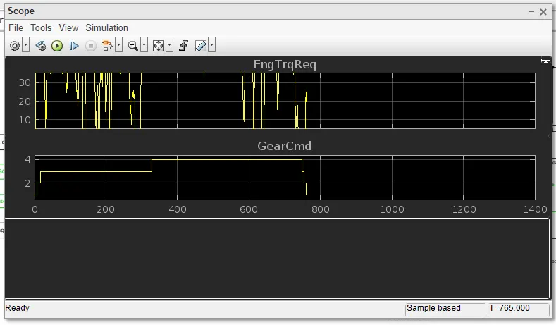
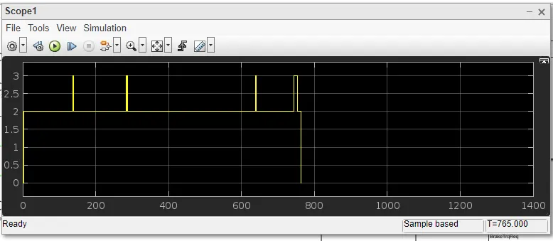
Controller Scope
Electric Motor Sope
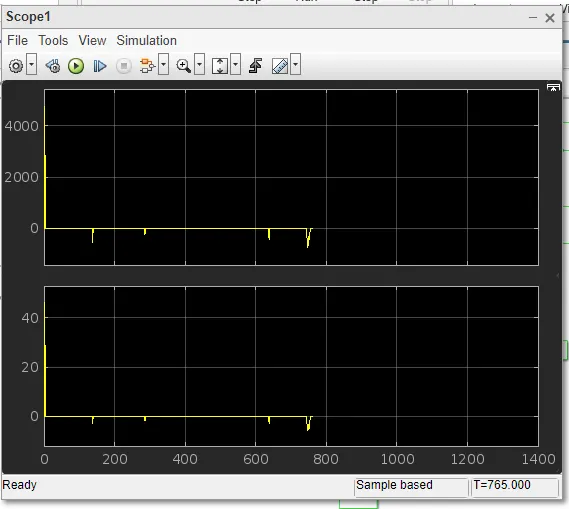
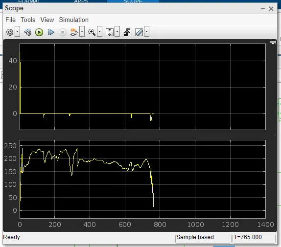
Engine Control Scope
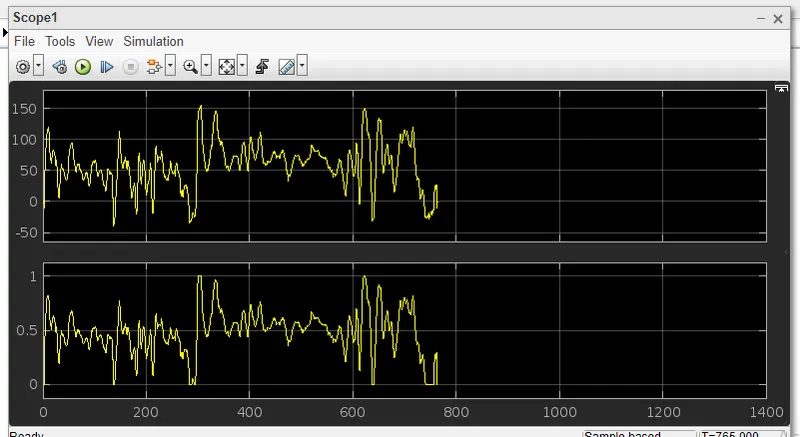
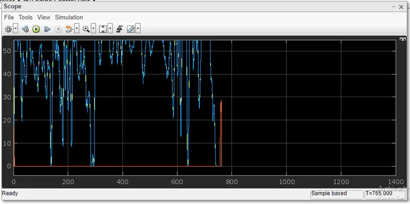
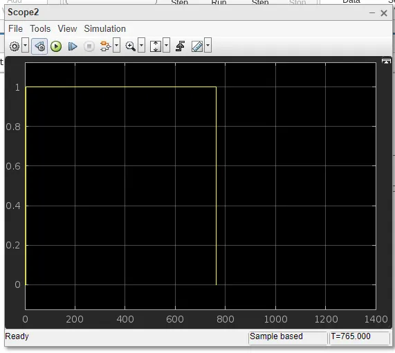
ESS Scope
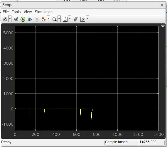
Idle Control Scope
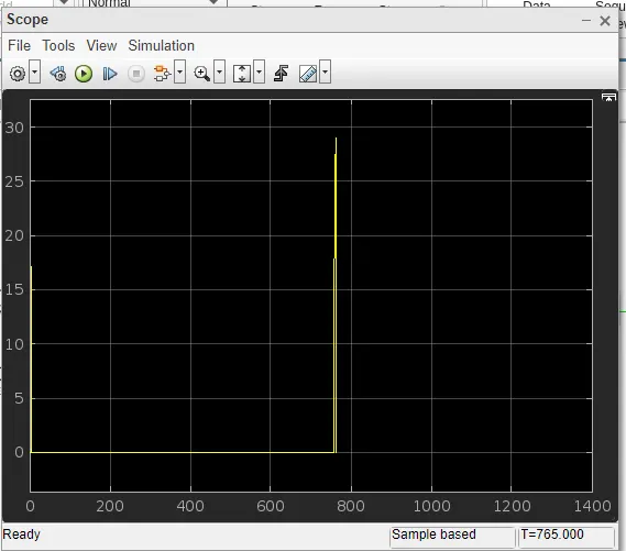
SOC Estimation Scope
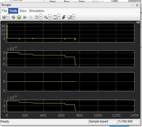
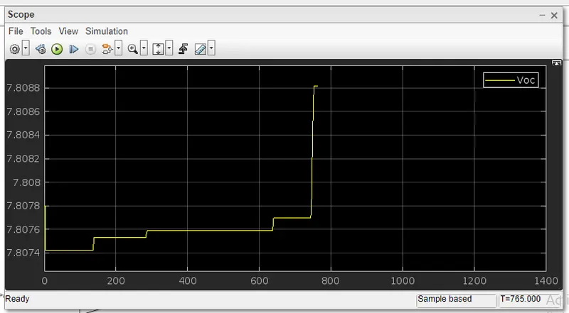
Terminal Voltage Scope
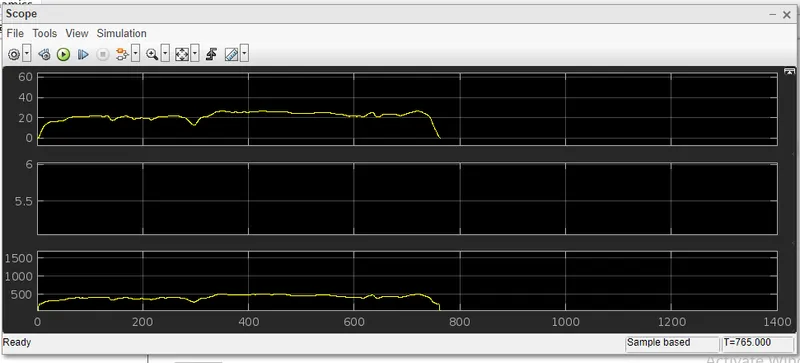
Vehicle Dynamic Scope
Conclusion:
The Various performance of characteristics and operating point of UDDS drive cycle and HWFET drive cycle are analysed and graphs are plotted.
Time trace for engine, Transmission input, Transmission output and wheelspeed with respect to time.
Engine torque, Engine power, Fuel rate and Fuel consumption with respect to time.
Accelerator and brake pedal, gear command and vehicle desired, actual speed, vehicle distance with respect to time.
Engine operating points on the engine fuel map with respect to time
Motor speed, Torque, Motor input power with respect to time.
Pack voltage, Current and State of charging with respect to time.
The motor operating points on the motor input power map with respect to time.
Please find below attached files for your reference