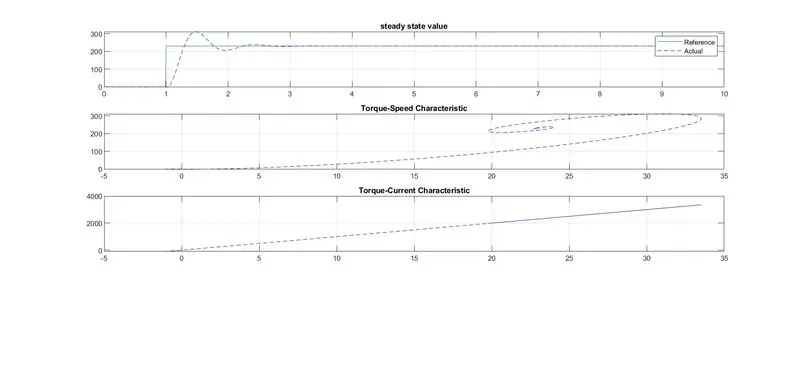
Project - Speed Control of a Direct Current (DC) motor
Aim: To design a PID controller for a DC Motor to control it's speed.
Key Highlights:
- Mathematical modeling from the first principles
- Modeling an Electrical Engineering system
- Simulink based modeling
- Control law design and test
- Stability of a dynamic system
Deliverables:
- Matlab script to define modeling and control design parameters
- Simulink model to simulate and verify the design
Theory: 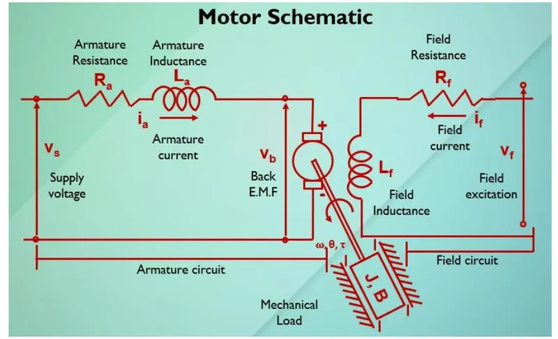
A DC motor is defined as a class of electrical motors that convert direct current electrical energy into mechanical energy.
Parts Of a DC Motor
- Armature or Rotor:The armature of a DC motor is a cylinder of magnetic laminations that are insulated from one another. The armature is perpendicular to the axis of the cylinder. The armature is a rotating part that rotates on its axis and is separated from the field coil by an air gap.
- Field Coil or Stator:A DC motor field coil is a non-moving part on which winding is wound to produce a magnetic field. This electro-magnet has a cylindrical cavity between its poles.
Working:
A magnetic field arises in the air gap when the field coil of the DC motor is energised. The created magnetic field is in the direction of the radii of the armature. The magnetic field enters the armature from the North pole side of the field coil and “exits” the armature from the field coil’s South pole side.The conductors located on the other pole are subjected to a force of the same intensity but in the opposite direction. These two opposing forces create a torque that causes the motor armature to rotate.
Mathematical Modelling Of DC Motor:
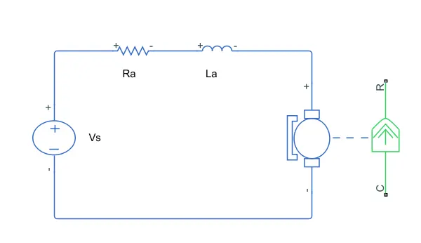
Circuit Diagram OF DC Motor
Differential Equation Pertaining to DC Motor:
J = Moment of Inertia of Rotor.
B = Damping Coefficient.
Ra = Armature resistance
La = Armature Inductance
Kb = Back emf constant
KT = Motor Torque Constant
V = Supply Voltage
Motor Torque T = KT * I
Back EMF Vb = Kb * ω = Kb * dθ/dt
Transfer function of output angle θ(s) to the input angle V(s) given by
Ga(s) = θ(s)/V(s) = KT / s[(Ls+R) * (Js+B) + (KT * Kb)]
Transfer function of output angle ω(s) to the input angle V(s) given by
Ga(s) = (s)/V(s) = KT / [(Ls+R) * (Js+B) + (KT * Kb)]
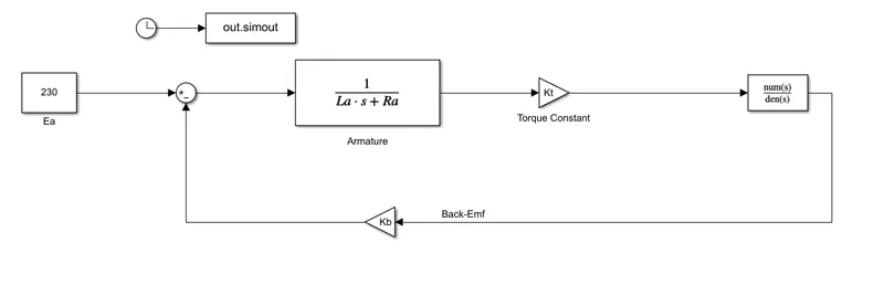
DC Motor Modelling.
State Space equations for the DC Motor
dI/dt = - (R/L) I + (1/L) V – (Kb/L) d/dt
dI/dt = - (R/L) I + (1/L) V – (Kb/L) ω dI/dt
dω/dt= - (B/J) ω + (1/J) KTI
Y(t) = ω = d/dt
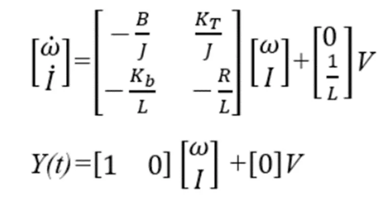
A state space representation of the DC motor from above equations
PID Controller:
Proportional-Integral-Derivative (PID) control is the most common control algorithm used in industry and has been universally accepted in industrial control.PID algorithm consists of three basic coefficients; proportional, integral and derivative which are varied to get optimal response.
The control design process begins by defining the performance requirements. Control system performance is often measured by applying a step function as the set point command variable, and then measuring the response of the process variable. Commonly, the response is quantified by measuring defined waveform characteristics. Rise Time is the amount of time the system takes to go from 10% to 90% of the steady-state, or final, value. Percent Overshoot is the amount that the process variable overshoots the final value, expressed as a percentage of the final value. Settling time is the time required for the process variable to settle to within a certain percentage (commonly 5%) of the final value. Steady-State Error is the final difference between the process variable and set point.
Proportional Response
The proportional component depends only on the difference between the set point and the process variable. This difference is referred to as the Error term. The proportional gain (Kc) determines the ratio of output response to the error signal. For instance, if the error term has a magnitude of 10, a proportional gain of 5 would produce a proportional response of 50. In general, increasing the proportional gain will increase the speed of the control system response. However, if the proportional gain is too large, the process variable will begin to oscillate. If Kc is increased further, the oscillations will become larger and the system will become unstable and may even oscillate out of control.
Integral Response
The integral component sums the error term over time. The result is that even a small error term will cause the integral component to increase slowly. The integral response will continually increase over time unless the error is zero, so the effect is to drive the Steady-State error to zero. Steady-State error is the final difference between the process variable and set point. A phenomenon called integral windup results when integral action saturates a controller without the controller driving the error signal toward zero.
Derivative Response
The derivative component causes the output to decrease if the process variable is increasing rapidly. The derivative response is proportional to the rate of change of the process variable. Increasing the derivative time (Td) parameter will cause the control system to react more strongly to changes in the error term and will increase the speed of the overall control system response. Most practical control systems use very small derivative time (Td), because the Derivative Response is highly sensitive to noise in the process variable signal. If the sensor feedback signal is noisy or if the control loop rate is too slow, the derivative response can make the control system unstable.

Stability of the system
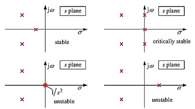
The location of poles in the s-plane decides the stability of the system. For a Bounded Input Bounded Output (BIBO) location of poles must be in LHP. If poles are on RHP then the system is unstable. If poles lie on jw axis then system is marginally stable.
PID controller for DC Motor
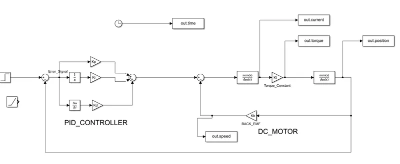
Design Parameters