Project - Speed Control of a Direct Current (DC) motor

Aim: To design a Simulink model for the DC motor shown in Figure 1. amd aslo by Using the Proportional, Integral, and Derivative (PID) control design knowledge gained in the training to design, develop and test a controller to maintain a desired speed for the motor.

Answer:

Here the Speed control of a DC motor is either done manually by the operator or by means of an automatic control device.

This is different to speed regulation where the speed is trying to be maintained or regulated against the natural change in speed due to a change in the load on the shaft

so the speed can be varied by changing:

The terminal voltage of the armature V

The external resistance in armature circuit Ra

The flux per pole

So Terminal voltage and external resistance involve a change that affects the armature circuit while flux involves a change in the maginetic field

so Therefore speed control of DC motor can be classified into:

Armature Control Methods

Field Control Methods

DC motor Parameters:

J=0.01; %Moment of Inertia of the rotor-kgm^2

B=0.1; %Motor viscous friction constant-Nms

Km=0.01; %Back EMF constant-V/rad/s

Kt=0.01; %Motor Torque constant-Nm/A

Ra=1; %Armature resistance-ohm

PID Design:
Basic eqn: u(t) = Kp*e(t) + Ki*int(e(t)dt) + kd*diff e(t)/dt
Modified eqn: Vs = Kp*(wref - w) + Ki*int((wref - w)dt) - Kd*Ia

Matrix A and B are found from the state space model of a DC motor,
(d/dt)*[teta_dot;i] = [-B/J Kt/J;-Km/La -Ra/La]*[teta_dot;i] + [0 1/La]*Vs

y = [1;0] * [teta_dot;i]

%Matrix - Plant model
A=[-B/J Kt/J;-Km/La -Ra/La];
C=[0;1/La];

%Poles
Matrix P is found from the open loop Transfer function of the DC motor denominator

Eqn: w(S)/Vs(S) = Kt/(J*La(S^2) + J*Ra+B*La(S) + B*Ra+Kt*Km)

P=roots([J*La J*Ra+B*La B*Ra+Kt*Km]);
K=place(A,C,P);

K= -1.4606e-15, 2.2204e-16

Script:
DC_motor_parameters.m
J=0.01; %Moment of Inertia of the rotor-kgm^2
B=0.1; %Motor viscous friction constant-Nms
Km=0.01; %Back EMF constant-V/rad/s
Kt=0.01; %Motor Torque constant-Nm/A
Ra=1; %Armature resistance-ohm
La=0.5; %Armature Inductance-Henry

%Matrix - Plant model
A=[-B/J Kt/J;-Km/La -Ra/La];
C=[0;1/La];
%Poles
P=roots([J*La J*Ra+B*La B*Ra+Kt*Km]);
K=place(A,C,P);

DC_motor_plot.m
close all;
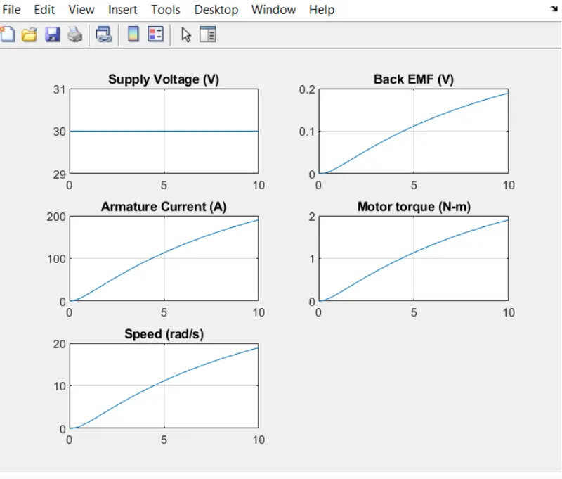
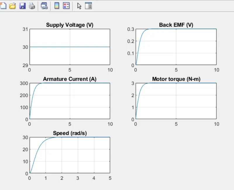
subplot(321);plot(out.time,out.vs);grid;title('Supply Voltage (V)');
subplot(322);plot(out.time,out.vb);grid;title('Back EMF (V)');
subplot(323);plot(out.time,out.ia);grid;title('Armature Current (A)');
subplot(324);plot(out.time,out.t);grid;title('Motor torque (N-m)');
subplot(325);plot(out.time,out.w);grid;title('Speed (rad/s)');

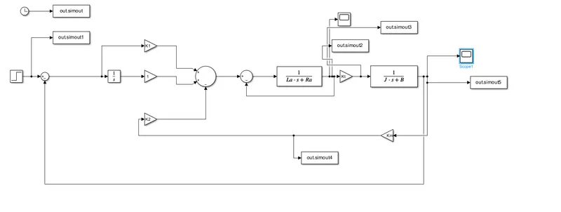
SCOPE:

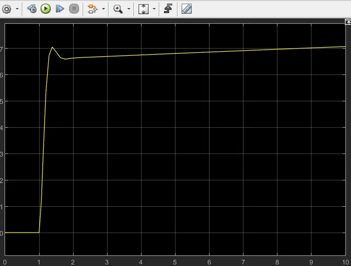
PLOT:

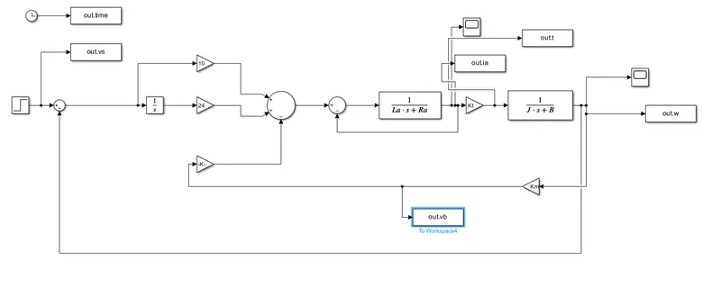
MODEL:2

After changing kp,kd,ki

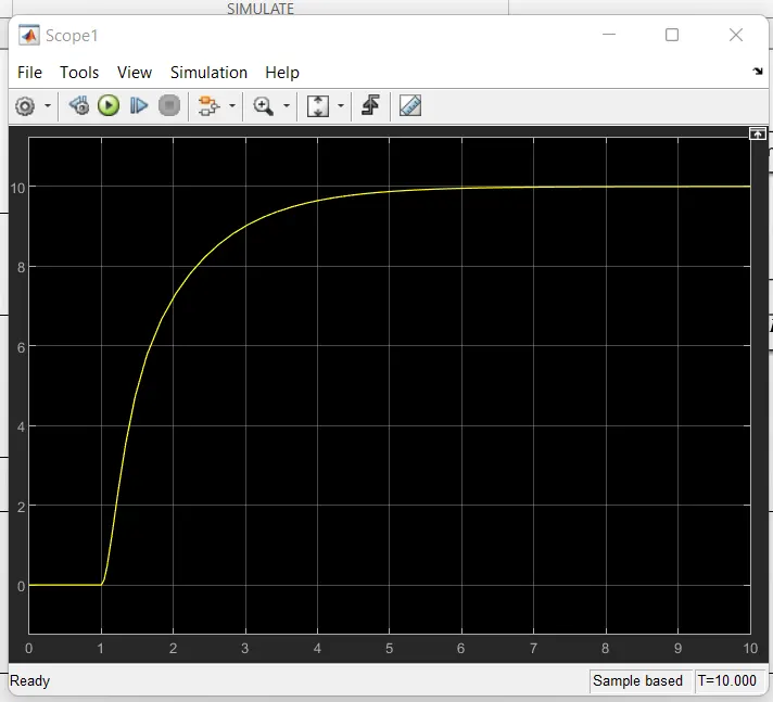
SCOPE:

PLOT:

CONCLISION:

Initially, the DC motor model was made and the values for PID design were calculated and the PID model was incorporated into the DC motor model. The supply voltage was set to 30 and the simulation time was 10s. The solver was set to Fixed-type and to be solved by ode4(Runge-Kutta method). The parameters of the dc motor were given. The poles were calculated using the place function and Ki was set to 1 and the model was run. The result was unstable and the required constant speed was not achieved. So, the next step was to iterate the values of Kp, Kd, and Ki to get a stable speed. After many iterations, the required stable speed was achieved with settling time <2s, Overshoot<5%, and Steady state error<1%. The found values were Kp=10;Kd=0.13;Ki=24;

Therefore, the speed of the dc motor was controlled and made to run at the desired speed.