Challenge

Project - Speed Control of a Direct Current (DC) motor

SSagar Kumar Barpete2 Nov 2022

Given Project: In this project, a Simulink model for the DC motor will be first developed per the schematic shown in the Figure and also Use the Proportional, Integral, and Derivative (PID) control design knowledge gained in the training to design, develop and test a controller to maintain a desired speed for the motor.

Solution:

To making a Simulation model with PID controller to regulate the speed of the DC Motor

Used Transfer function as per video instruction

By converting transfer function to state space we got

Then setting up some Parameters for the simulation function as -

J = 0.01; % Moment of Inertia of the rotor in kg-m^2

B = 0.1; % Motor viscous friction constant in N-m-s

Km = 0.01; % Back EMF constant in v/rad/s

Kt = 0.01; % Motor torque constant in N-m/amp

Ra = 1.0; % Resistance of the armature circuit in ohms

La = 0.5; % Inductance of the armature circuit in henries

Setting up some Paramenters for PID system for DC Motor as -

% As in Control Design Objectives should be

Setting time < 2s

Overshoot < 5%

Steaady state error < 1%

hence,

k = 3944.0; % stiffness constant of the spring-mass system

wn = 6.2832; % sqrt(k/m) rad/s

fn = 1.0; % wn/(2*pi) Hz

zeta = 0.5; % Under damped system design

p1 = -zeta*wn+wn*sqrt(zeta^2-1);

p2 = -zeta*wn-wn*sqrt(zeta^2-1);

p = [p1;p2];

A = [-B/J Kt/J; -Km/La -Ra/La];

D = [0; 1/La];

K = place(A,D,p); % Kp & Kd gains are obtained from an earleier design using PLACE command

% Kp & Kd gains are obtained and used in simulation as K(1) and K(2)

Ki = 0.01; % different values as Ki = 0.10;

Simulation model used :

Blocks and Logics Used in Simulink model:

Clock - To Provide Simulation time to function

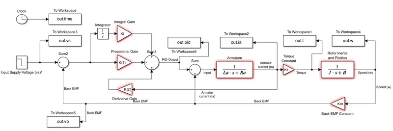
To Workspace - To log data to workspace from Simulink model for Like: out.time, .vs, .vb, .pid, .ia, .t, .w

Sum - To provide addition and subtract operation to model

Gain - To multiply inputs with different conditions

Step - To use step function as input supply with different confugrations

Integrator - To perform Integration function to model

Transfer Fcn - Model linear system by transfer function

With configuration as Fixed type solver with Fixed step size of 0.01 for stop time of 10 seconds

Model Processing and results observation with different values

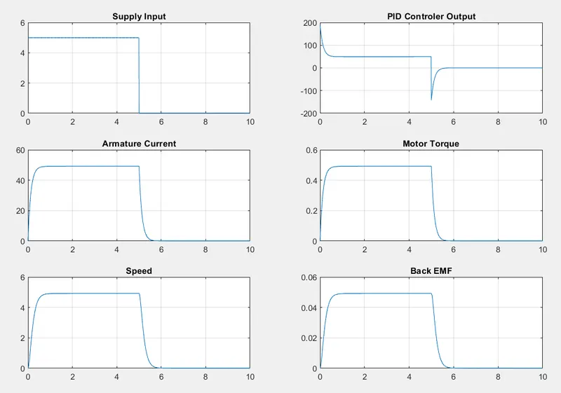
01. with Ki = 0.01 and step input as step time = 5, Initial value = 5 and Final value = 0

Result plot

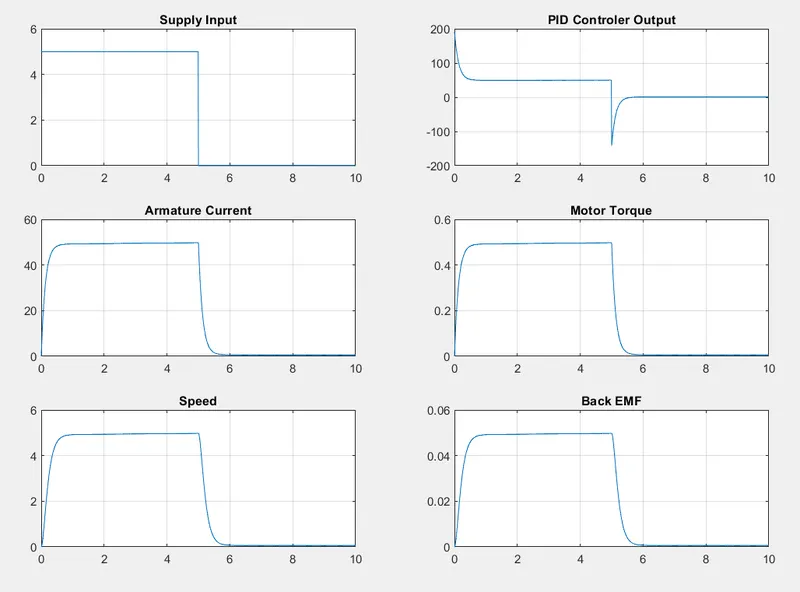
02. with Ki = 0.10 and step input as step time = 5, Initial value = 5 and Final value = 0

Result plot- Observed slight changes by changing value of Ki (integral gain)

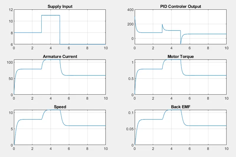
03. with Ki = 0.10 and using two step blocks as input to give input as pulse wave to observe different output and its variations for same simulation model

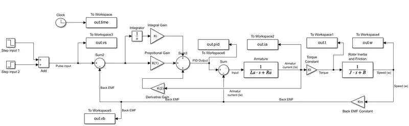
with step input 1 as step time = 5, Initial value = 5 and Final value = 0 and step input 2 as step time = 3, Initial value = 3 and Final value = 6

Observed result plots

Commands used to plot above plots are

close all;

subplot(321);plot(out.time,out.vs);grid;title('Supply Input');

subplot(322);plot(out.time,out.pid);grid;title('PID Controler Output');

subplot(323);plot(out.time,out.ia);grid;title('Armature Current');

subplot(324);plot(out.time,out.t);grid;title('Motor Torque');

subplot(325);plot(out.time,out.w);grid;title('Speed');

subplot(326);plot(out.time,out.vb);grid;title('Back EMF');

Project - Speed Control of a Direct Current (DC) motor

Ship work like this
in your own course.

Talk to a career counsellor

Ship work like thisin your own course.

Talk to a career counsellor

Ship work like this
in your own course.