Project - Position control of mass spring damper system

Aim: to obtain the transfer function of spring mass damper system using PID controller to match with input.

Objectives:

• using kp,ki,kd the output should match with input.
• implimenting spring mas damper equation in transfer function observe the displacement.

Theory:

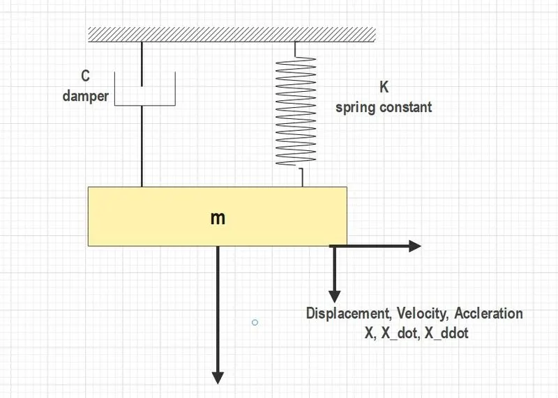
Spring mass damper system:

F(t) = m*x_double dot + c x_dot + kx

where,

m = mass

k = spring stiffness constant

x = displacement

x_dot = velocity

x_double dot = accleration

if we apply laplace transform to above diffrential equation,

F(s) = ms^2 + csX(s) + Kx(s)

F(s) = (ms^2 + cs +X(s)

Transfer Function F(t) :

=X(s)/F(s)

= 1/ms^2 + cs +k

=1/m/(s^2 + cs/m+k/m)

=k/s^2 + 2*zeta*wn+wn^2

by comparing above eqution we obtain relation:

k =1/m; 2*zeta*wn=c/m; wn^2 = k/m; or wn = sqrt k/m ; zeta = c/2*sqrt m*k ; -zeta*wn±wn*sqrt zeta^2-1

Control System Design:

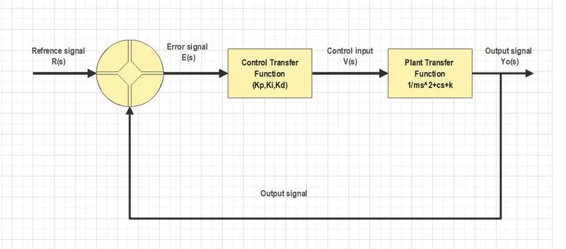
• Refrence signal R(s): it is the input signal of the system.

• Error signal E(s): difference between input and output signal is known as error signal.

• Control input signal V(s): after rectification generated required output is known as control input signal.

• Output signal o(s): output signal is the signal generated by system with given input.

• Error junction: compares output with input and generates error signal.

• Control transfer function: control input genereated by this transfer function to stablize the system with given input.

• Plant transfer function: spring mass equation implemented in this function it has transfer function 's' .

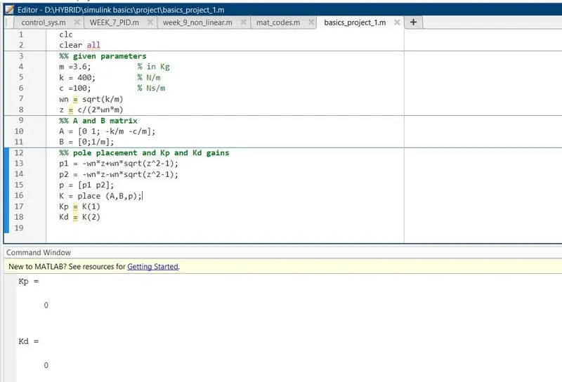
Matlab code implementation:

clc
clear all
%% given parameters
m =3.6;          % in Kg
k = 400;         % N/m
c =100;          % Ns/m
wn = sqrt(k/m) 
z = c/(2*wn*m)
%% A and B matrix
A = [0 1; -k/m -c/m]; 
B = [0;1/m];
%% pole placement and Kp and Kd gains
p1 = -wn*z+wn*sqrt(z^2-1);
p2 = -wn*z-wn*sqrt(z^2-1);
p = [p1 p2];
K = place (A,B,p);
Kp = K(1)
Kd = K(2)

Result:

Simulink Model:

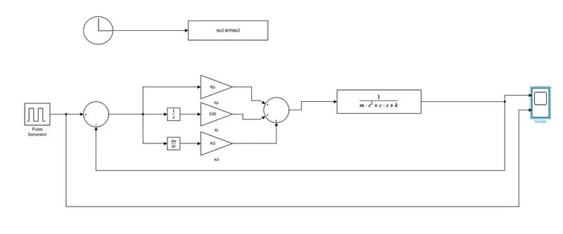
Model implementation:

• using following blocks and gains we have created the model-

1. clock
2. to workspace
3. circular summing junction
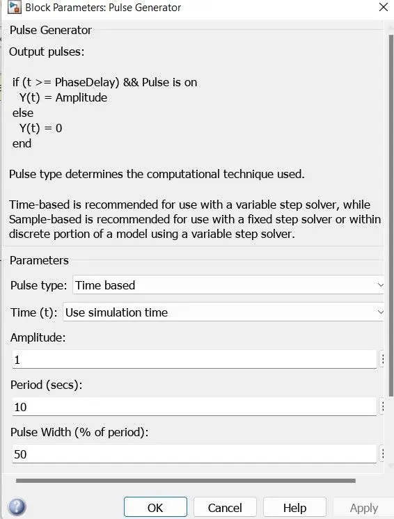
4. pulse generator
5. gain blocks
6. integrator
7. derivative
8. transfer function
9. scope

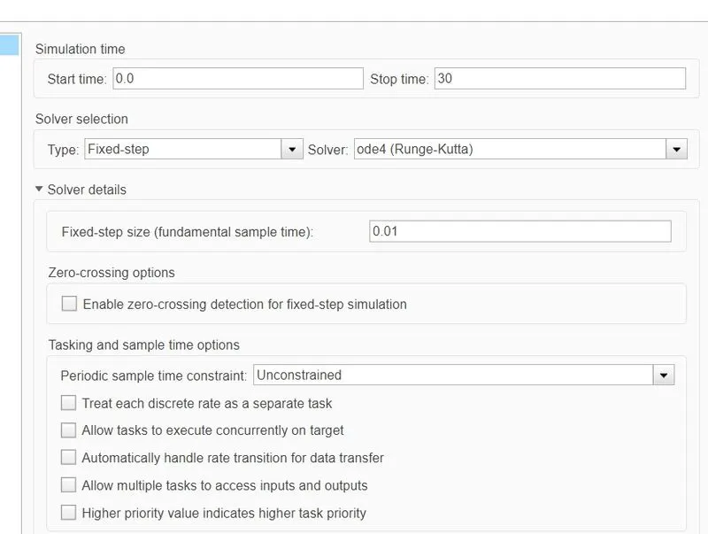
• by using following method we have build and ran simulink model and we obtain results as follows -

pulse parameters:

results:

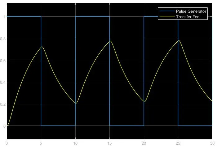
changing value of Ki = 100

when we set ki value = 100 we can observe in following graph system output does not match with input.

where pulse generator is input and transfer function is output.

that also means system is bheaving as a under damped system.

below system is observed As a under damped system(zeta<1).

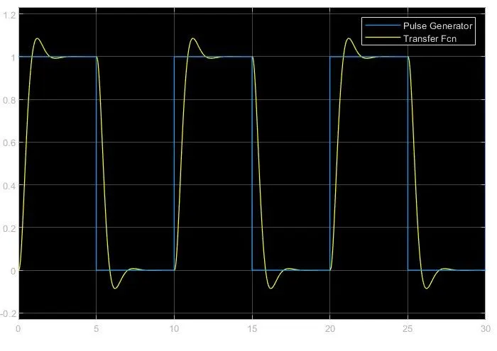
changing value of Ki = 1000

when we set ki value = 1000 we can observe in following graph system that system output overshoot above 1 and undershoot at below one and then slightly match with input after that again stable output observed.

where pulse generator is input and transfer function is output.

that also means system is bheaving as a overdamped system.

below system is observed As a overdamped system( zeta>1).

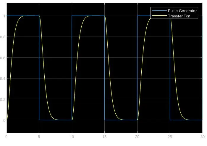
changing value of Ki = 500

in order to achive stable system behaviour we have changed the value of ki manually.

after changing values 3 to 4 times ki = 500 is the value at which our output follows input.

when we set ki value = 500 we can observe in following graph system output does match exactly with input.

output is smoothly follows input without any overshoot and undershoot.

below system is observed As a critically damped system(zeta=1).

conclusion:

• by changing value of ki mnually system can be analyse whether system is in underdamped, overdamped and critically damped.
• system bheviour can be tracked as well using transfer function.
• linearization of system can be achived by using diffrent refrence input.
• kp,ki,kd gain act as a close loop feedback system.
• summing junction compares input with output and then tranfer the signal.