Project - Position control of mass spring damper system

• The values are calculated by running a matlab script as shown below.
• The pole values obtained are used to determine the Gain control value (Kp and Kd) by using the 'place' command.
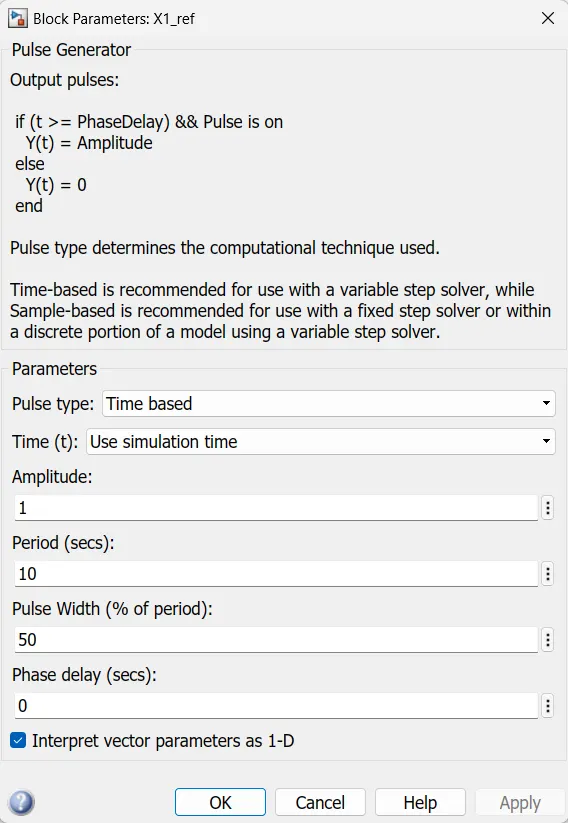
• The model is simulated for different values of the Integral gains (Ki) and the response is analyzed with respect to the reference signal. The reference signal values are as shown below.

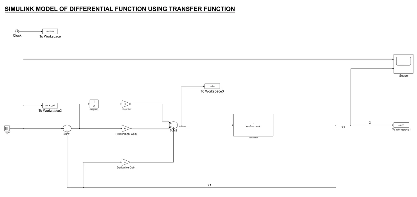
• The Displacement of the system is determined using the formula shown below. The simulink model design is created based on the same formula shown below.
  X1_dot = X2
  X2_dot = (-k/m)*X1 + (1/m)*u
  X2_dot = (-k/m)*X1 + (1/m)*[Kp*(X1ref - X1) - Kd*X2 + Ki*int(X1_ref - X1)*dt]
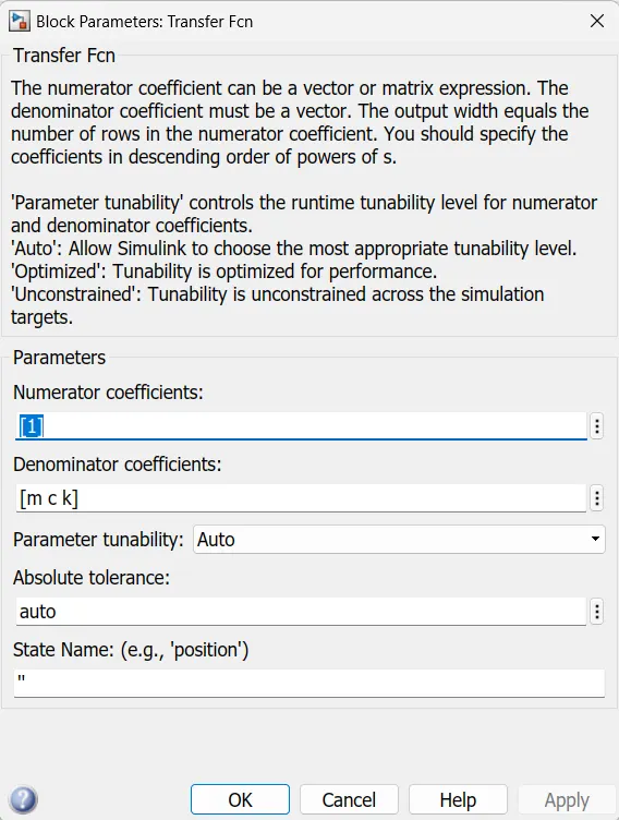
• The transfer function for a spring mass damper system is 1 / ( m * s^2 + c * s + k )
  

where the value of mass (m) , damping coefficient (c) , spring constant (k)

m = 3.6 kg

k = 400 N/m

c = 100 Ns/m

these values of m , c , k are given in the denominator as the differential order ( high to low )

where numerator will be 1

• A Transfer function block is used to calculate the transfer fucntion of the spring mass damper system. The block setting are shown in the figure below.

MATLAB CODE :

% Determination of the Gain control for the Transfer function in the spring mass damper system 
clear
close
clc

% Inputs
m = 3.6;
c = 100;
k = 400;
fn = 1;
wn = sqrt(k/m);


% Design parameters
zeta = 0.5;

p1 = (-zeta*wn) + wn*sqrt(zeta^2 - 1);
p2 = (-zeta*wn) - wn*sqrt(zeta^2 - 1);
P = [p1;p2]

% Matrix inputs
A = [0 1; -k/m c/m];
B = [0 ; 1/m];

% Kp and Kd gains are obtained from the earlier design using the Place
% command
K = place(A,B,P)
Kp = K(1);
Kd = K(2);
Ki = 1000;

% Dynamics
% X1_dot = X2
% X2_dot = (-k/m)*X1 + (1/m)*u
% X2_dot = (-k/m)*X1 + (1/m)*[Kp*(X1ref - X1) - Kd*X2 + Ki*int(X1_ref - X1)*dt]

Model :

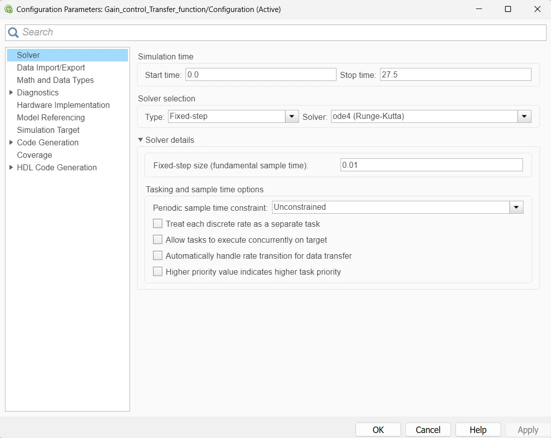
Model Settings :

Output :

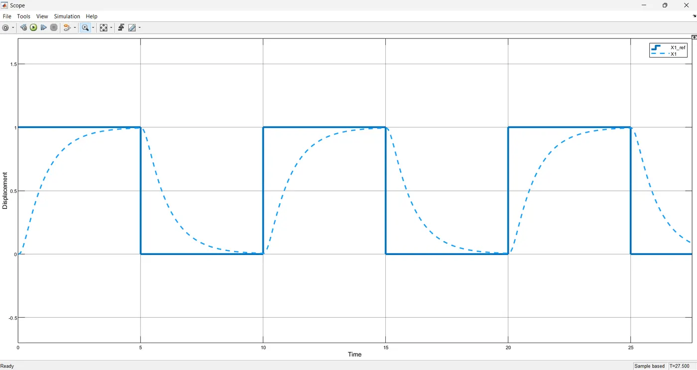
Integral Gain (Ki) = 500

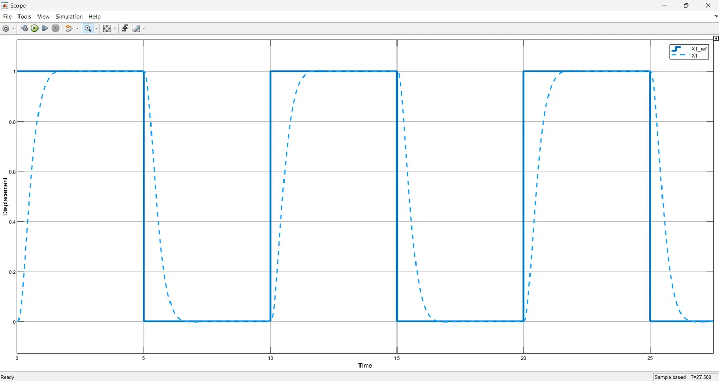
Integral Gain (Ki) = 1000

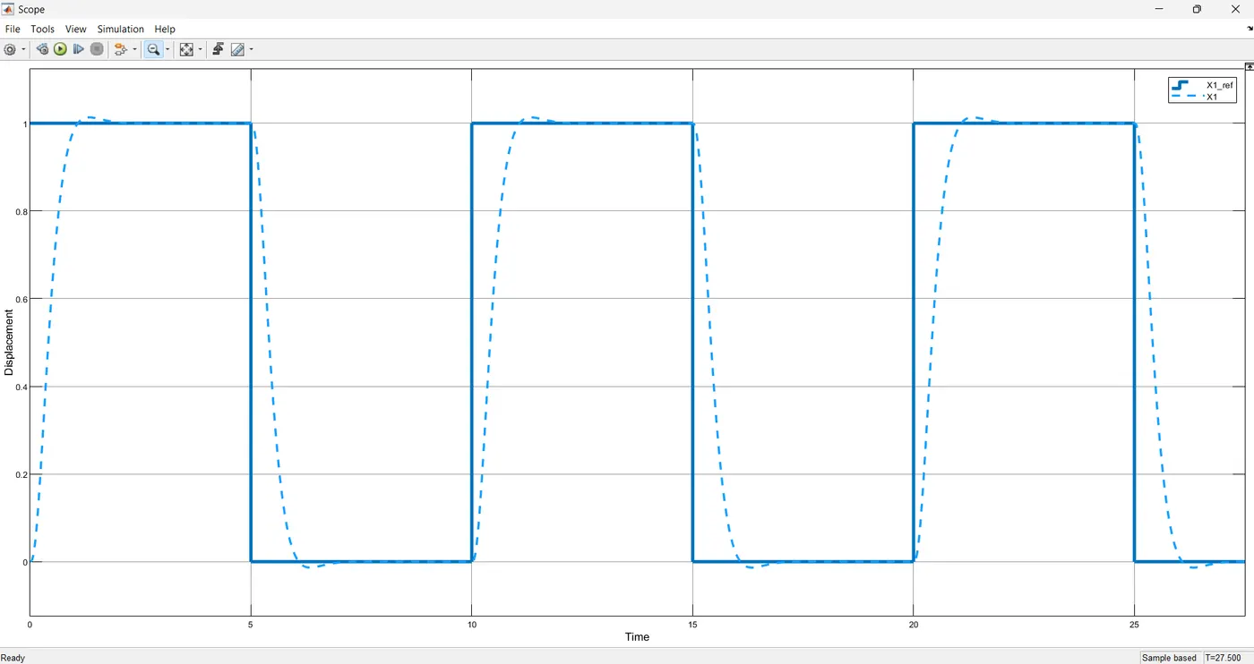
Integral Gain (Ki) = 1300

Conclusion :

• The above Simulink model is used to replicate the PID controller containing the Feedback Control Gains (Kp, Kd and Ki).
• The Xref value is obtained from the pluse 'pluse generator' block with the magnitude of 1.0 for the time period of 5 seconds and the total simulation time is fixed as 27.5 seconds.
• The values of the Proportional and the Derivative Control Gains are obtained using the place command in the MATLAB Script.
• The response of the Controller is obtained for the different values of the Integral Gain controller.
• Transfer Function block is used to calculate displacement (X1) which is required to maintain the reference displacement (X1_ref) values.
• The results are recorded and are shows that as the values of the Integral Gain controller is increased the overall response and stability of the output was improved.