Project - Position control of mass spring damper system
[NOTE : HERE I SHOULD BE WHAT I AM UNDERSTAND THE CONCEPT THAT'S MENTION AND MORE OVER DETAILS REFERENCE ADDED FROM BASED ON ONLINE REFERENCE ARTICULES ATTACHED FOR MORE CLARIFICATION]
QUESTION :
Obtain the transfer function of a mass spring damper system and use it in the model. Add a PID controller to adjust the force on mass so that its position follows a reference signal.
Take m = 3.6; %kg k = 400; %N/m c = 100; %Ns/m
ANSWER :
ANSWER I SPLITTED TO 2 TYPES BASED ON BELOW LIKE,
UNDER DAMEPED SYSTEM Z= 0.5
MORE DAMPED BEHAVIOUR SYSTEM Z = 0.9
AIM :
To Obtain the transfer function of a mass spring damper system and use it in the model. Add a PID controller to adjust the force on mass so that its position follows a reference signal.
Take m = 3.6; %kg k = 400; %N/m c = 100; %Ns/m
Mass Spring Damper System
Transfer function and state space model are developed for system shown below.
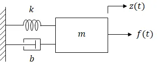
| (input) | f(t) | = | external force applied on mass | |
| (output) | z(t) | = | position | unknown |
| m | = | mass | ||
| k | = | spring constant | ||
| b | = | damping coefficient |
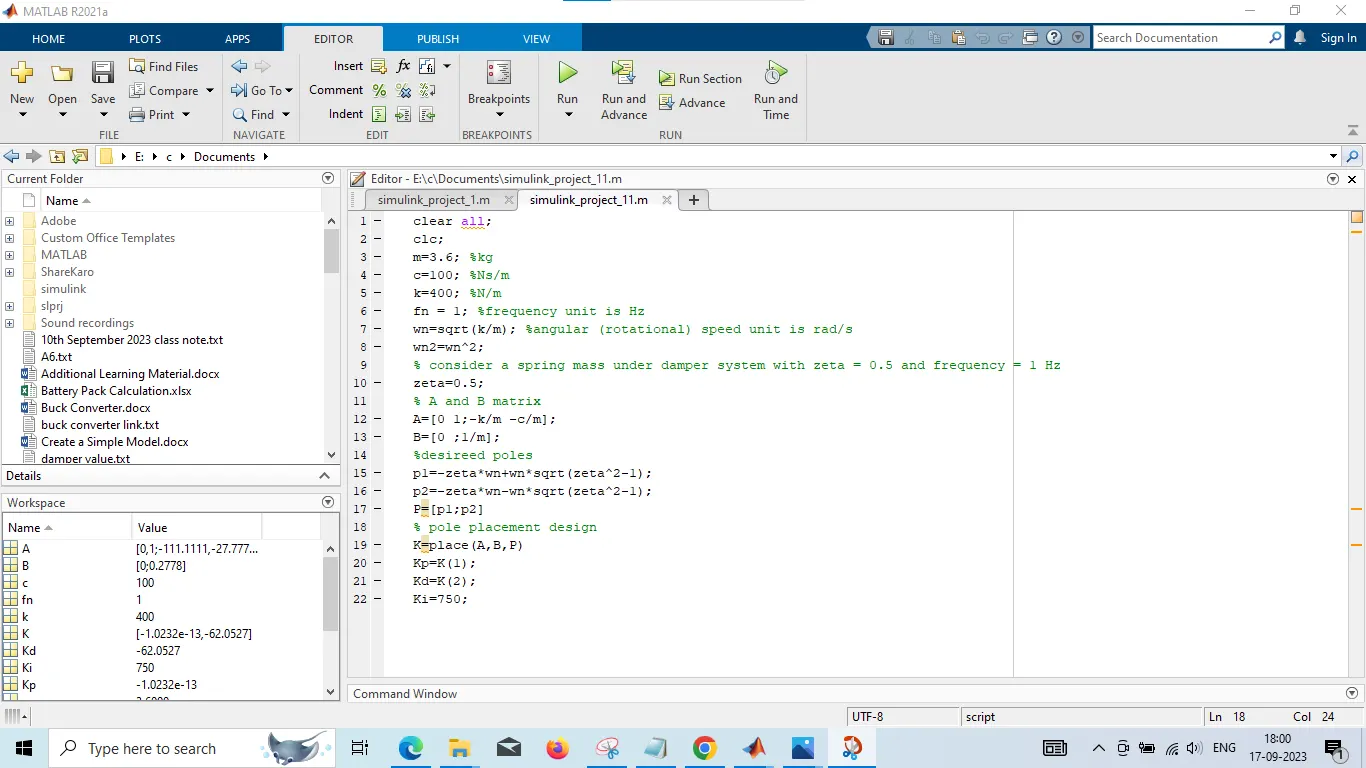
Differential Equation
1 unknown so 1 equation is needed.
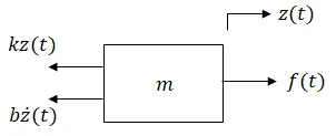
Newton's 2nd law:
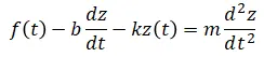
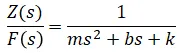
Transfer Function
Laplace transform (eq. 1):

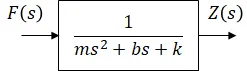
Solve for Z(s)/F(s):
Block Diagram
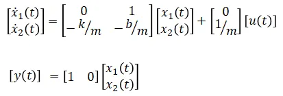
State Space Model
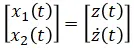
When there is a mass in a system, its position and velocity are commonly chosen as state variables. Also, position, velocity, and force (input) are sufficient to determine this system's future position (output). For these reasons, position and velocity are chosen as state variables.
State vector:
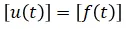
Input vector:
Output vector:

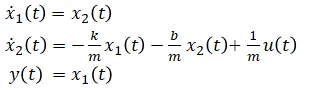
Rewrite (eq. 1) in these new notations:

Rearrange equations to express ẋ(t) and y(t) in terms of x(t) and u(t):
Organize into matrix format:
SIMULINK :
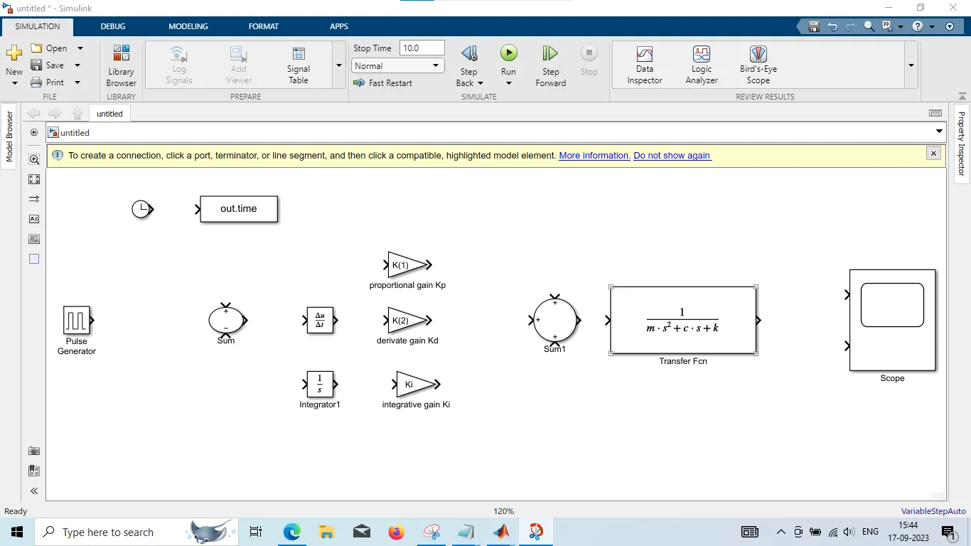
USED BLOCK DETAILS :
Scope - Display signals generated during simulation
The Simulink Scope block and DSP System Toolbox Time Scope block display time domain signals.
Add - Add or subtract inputs
The Sum block performs addition or subtraction on its inputs.
Add, Subtract, Sum of Elements, Sum :
The Sum block performs addition or subtraction on its inputs. The Add, Subtract, Sum of Elements, and Sum blocks are identical blocks. This block can add or subtract scalar, vector, or matrix inputs. It can also collapse the elements of a signal and perform a summation.Add or subtract inputs
Integrator - Integrate signal
The Integrator block outputs the value of the integral of its input signal with respect to time.
Gain - Multiply input by constant
The Gain block multiplies the input by a constant value (gain).The input and the gain can each be a scalar, vector, or matrix.
You specify the value of gain in the Gain parameter. The Multiplication parameter lets you specify element-wise or matrix multiplication. For matrix multiplication, this parameter also lets you indicate the order of the multiplicands.
Gain is converted from doubles to the data type specified in the block mask offline using round-to-nearest and saturation. The input and gain are then multiplied, and the result is converted to the output data type using the specified rounding and overflow modes.
Integrator :
Integrate signal.The Integrator block outputs the value of the integral of its input signal with respect to time.If the integrator limits its output (see Limiting the Integral), the initial condition must fall inside the integrator's saturation limits. If the initial condition is outside the block saturation limits, the block displays an error message.
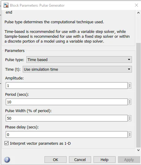
Pulse Generator
Generate square wave pulses at regular intervals.The Pulse Generator block generates square wave pulses at regular intervals. The block waveform parameters, Amplitude, Pulse Width, Period, and Phase delay, determine the shape of the output waveform. The following diagram shows how each parameter affects the waveform.
UNDER DAMEPED SYSTEM Z= 0.5 :
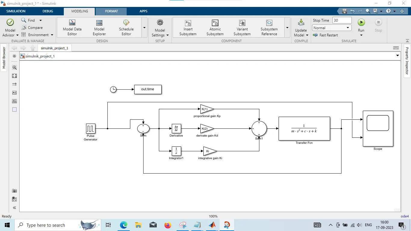
here
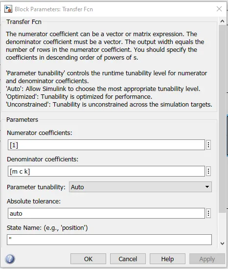
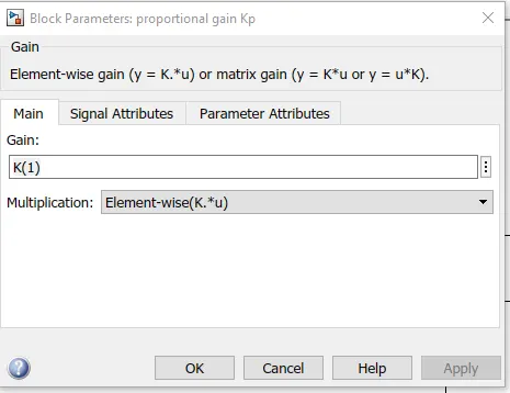
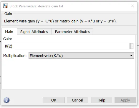
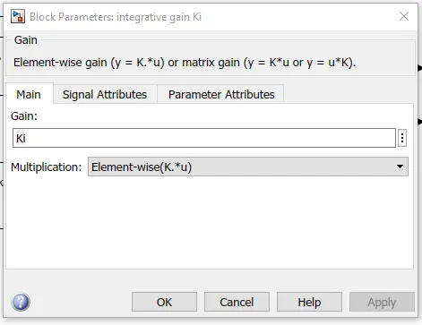
PULSE GENERATOR give reference input add to using sum block.proportional gain Kp[K(1)] get from ouput of sum block.derivative gain Kd[K(2)] derivate using devative block value get from sum block integrative gain Ki integrate using ingrator block value get from sum block.Kp,Kd,Ki gain output value add to sum 1 block.output of sum1 block value to transfer based formula[1/(m.s^2+c.s+k)] using tramsfer fcn block in this output value give to scope block and also pulse generator input directly connect with scope
PULSE GENERATOR INPUT :
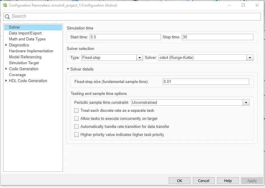
once simulink built than configuraion to
TRANSFER FUNCTION :
PROPORTION GAIN Kp :
DERIVATIVE GAIN Kd :
INTEGRATIVE GAIN ki :
once configuration finish save and run the simulink file check the ouput result in scope
OUTPUT RESULT :
zeta = 0.5
STOP TIME = 30 SEC
SCOPE :
SIMULINK :
USED BLOCK DETAILS :
Scope - Display signals generated during simulation
The Simulink Scope block and DSP System Toolbox Time Scope block display time domain signals.
Add - Add or subtract inputs
The Sum block performs addition or subtraction on its inputs.
Add, Subtract, Sum of Elements, Sum :
The Sum block performs addition or subtraction on its inputs. The Add, Subtract, Sum of Elements, and Sum blocks are identical blocks. This block can add or subtract scalar, vector, or matrix inputs. It can also collapse the elements of a signal and perform a summation.Add or subtract inputs
Integrator - Integrate signal
The Integrator block outputs the value of the integral of its input signal with respect to time.
Gain - Multiply input by constant
The Gain block multiplies the input by a constant value (gain).The input and the gain can each be a scalar, vector, or matrix.
You specify the value of gain in the Gain parameter. The Multiplication parameter lets you specify element-wise or matrix multiplication. For matrix multiplication, this parameter also lets you indicate the order of the multiplicands.
Gain is converted from doubles to the data type specified in the block mask offline using round-to-nearest and saturation. The input and gain are then multiplied, and the result is converted to the output data type using the specified rounding and overflow modes.
Integrator :
Integrate signal.The Integrator block outputs the value of the integral of its input signal with respect to time.If the integrator limits its output (see Limiting the Integral), the initial condition must fall inside the integrator's saturation limits. If the initial condition is outside the block saturation limits, the block displays an error message.
Pulse Generator
Generate square wave pulses at regular intervals.The Pulse Generator block generates square wave pulses at regular intervals. The block waveform parameters, Amplitude, Pulse Width, Period, and Phase delay, determine the shape of the output waveform. The following diagram shows how each parameter affects the waveform.
MORE DAMEPED BEHAVIOUR SYSTEM Zeta= 0.9 :
here
PULSE GENERATOR give reference input add to using sum block.proportional gain Kp[K(1)] get from ouput of sum block.derivative gain Kd[K(2)] derivate using devative block value get from sum block integrative gain Ki integrate using ingrator block value get from sum block.Kp,Kd,Ki gain output value add to sum 1 block.output of sum1 block value to transfer based formula[1/(m.s^2+c.s+k)] using tramsfer fcn block in this output value give to scope block and also pulse generator input directly connect with scope
PULSE GENERATOR INPUT :
once simulink built than configuraion to
TRANSFER FUNCTION :
PROPORTION GAIN Kp :
DERIVATIVE GAIN Kd :
INTEGRATIVE GAIN ki :
once configuration finish save and run the simulink file check the ouput result in scope
OUTPUT RESULT :
zeta = 0.9
STOP TIME = 30 SEC
SCOPE :
CONCLUSION :
To Simulink model like the one presented in the slides with feedback control gains.
Re-design the control gain, K, for a ζ of 0.5(under damping system and 0.9(also called more damping behaviour) and analyze the response for a pulse reference signal.
answer and result file find and atteched to file