Project - Position control of mass spring damper system

Answer: 

Spring-Mass-Damper system:

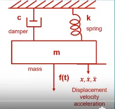
The differential equation representing the spring-mass-damper system shown above is given as:

   OR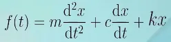 

where,

'm' is the mass

'C' is the damping coefficient

'K' is the stiffness or spring constant

'x' --> displacement

'x_dot' --> velocity

'x_dot_dot' --> acceleration

If we apply Laplace transform to the above differential equation, we get: 

F(s) = m*s^2* X(s) + c*s*X(s) + k*X(s)

F(s) = (m*s^2 + c*s + k)* X(s) 

X(s)/F(s) = 1 / (m*s^2 + c*s + k)  --------- I 

Above is the Transfer function of a Spring-Mass-Damper system. 

Standard second-order transfer function is given by     

X(s)/F(s) = K / (s^2 + 2*zeta*wn*s + wn^2)   ---------- II

If we compare above equation no. I & II, we get 

K = 1/m     

2*zeta*wn = c/m

wn^2 = k/m

Matlab script: 

% Parameters of mass spring damper system
m = 3.6; % mass kg
k = 400; % spring constant N/m
c = 100; % damping coeffiecient Ns/m

% Pole placement design
wn = sqrt(k/m); % Natural frequency in rad/s

% A & B matrix value

A = [0 1; -k/m -c/m];
B = [0; 1/m];

% Design values
zeta = 0.8; % for an under-damped behavior

% Placement of poles
p1 = -zeta*wn + wn*sqrt(zeta^2-1);
p2 = -zeta*wn - wn*sqrt(zeta^2-1);
P= [p1;p2];

K = place (A,B,P)    %Kp & Kd values are obtained. Kp = K(1), Kd = K(2)

Kp = 9000;    % Gain adjusted manually for optimum performance
Kd = 180.0;    % Gain adjusted manually for optimum performance
Ki = 12500;    % Gain adjusted manually for optimum performance

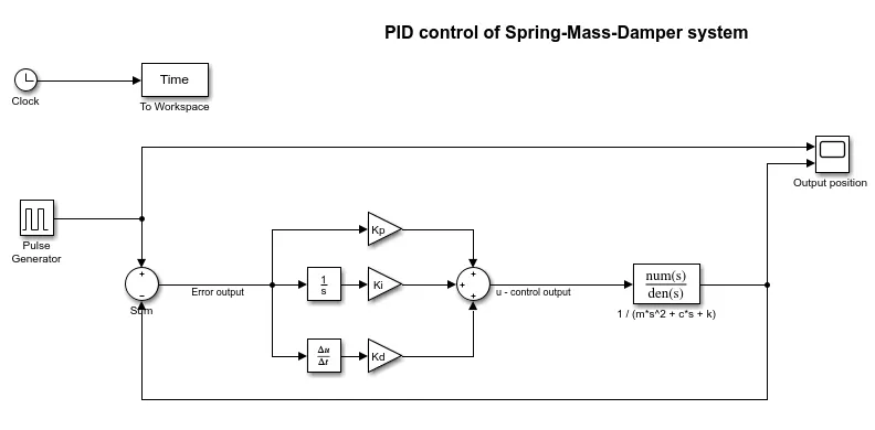
Simulink model: 

The simulink model shall be created using pulse generator, sum, gain, transfer function, integrator, scope , derivative, clock, workspace blocks

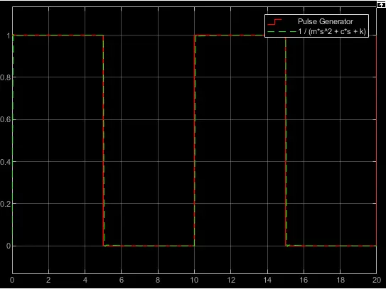
Tracking response: 

Conclusion: 

The control system objectives of Rise time, Settling time, Overshoot and Steady state error are achieved by using PID control method. Thus optimum tracking response is achieved.