Project - Position control of mass spring damper system
Simulink Basics Project- Position control of mass spring damper system
Problem: Obtain the transfer function of a mass spring damper system and use it in the model. Add a PID controller to adjust the force on mass so that its position follows a reference signal.
Take m = 3.6; %kg k = 400; %N/m c = 100; %Ns/m
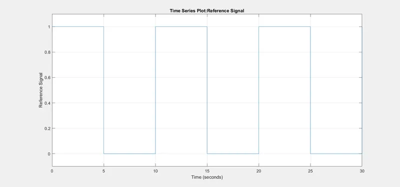
The reference signal is shown in the following figure.
Solution:
We know that the differential equation describing a Mass-Spring-Damper (MSD) system can be written as
`m(d^2x)/(dt^2)+c(dx)/(dt)+kx=f(t)` (1)
Where 'm' is the mass of the system,'c' is the damping co-efficient and 'k' is the stiffness/spring constant, 'x' is the displacement or position of the system, and 'f(t)' is the applied force on the system.
In s-domain, the transfer function between the displacement and the applied force can be written as
`G(s)=(X(s))/(F(s))=(1/m)/(s^2+(c/m)s+k/m)`, Laplace transformation ignores the initial conditions.
When we compare this with the standard 2nd order transfer function we can write `w_n=sqrt(k/m)`, where `w_n` is the natural angular frequency of oscillation of the system in rad/s, and `zeta=c/(2*sqrt(m*k))` where `zeta`is the damping ratio of the MSD system.
According to the given problem statement, we have considered the mass of system to be m=3.6 kg,k=400 N/m, and c= 100 N-s/m.

When this script is run we obtain the following result
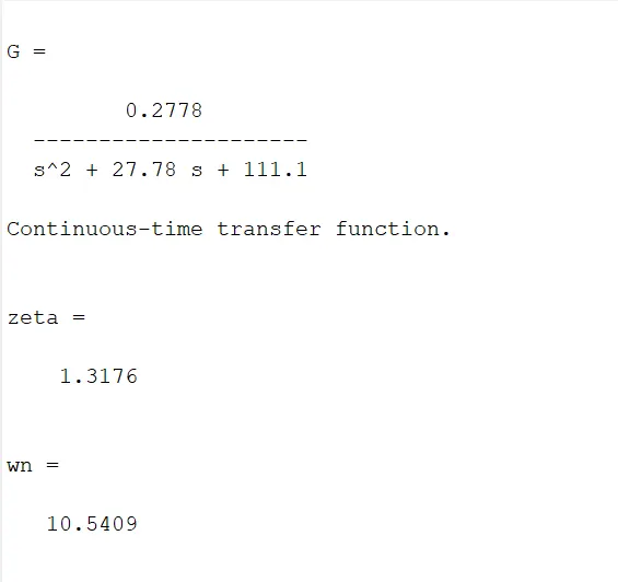
Therefore we get `w_n=10.5409`rad/s, and the damping ratio of the open loop MSD system is `zeta=1.3176`(overdamped in nature)
From Eq. (1) the state space representation of the MSD system can be derived as follows:
Let, `x_1=x`,f(t)=u, and y=x ['u' is the input, and 'y' is the output of the system]
`dotx_1=dotx=x_2` (2)
`dotx_2=-(k/m)x_1-(c/m)x_2+(1/m)u` (3)
Basically the displacement and the velocity are the states if the system and can be written as X=[x1;x2]
Therefore the state matrix A can be written as A=[0 1;-k/m -c/m]
The input matrix B can be written as B=[0;1/m]
The output matrix C=[1 0]
The transfer matrix D=[0]
The state equation is : dX/dt=AX+Bu (4)
The output equation is : y=CX+Du (5)
The main goal of our controller design is to get a feedback PID control law u=-K*X such that the state 'X' is driven to the origin from any non-zero initial condition or track a given reference signal starting from zero initial condition.
If we substitute the control law into the state equation we get
dX/dt=(A-B*K)X (6)
If we can select the gain matrix K such that the eigen values of the matrix (A-BK) are negative real with or without imaginary parts, then our design objective can be met.
In this example, the damping ratio of the MSD system is 1.3176, therefore whenever we apply any forcing function on the system, we can observe an overdamped slow response.
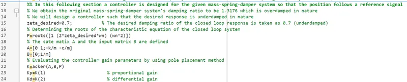
Therefore in order to make the system response faster and to follow a reference input, we will design the controller gain K in such a way that the overall closed loop system becomes underdamped, we used here ζ of 0.7.
The Matlab script file for the controller design section is given below
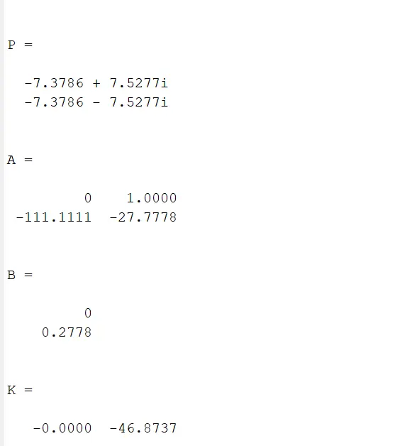
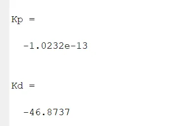
Following are the results when this script is simulated
The characteristic equation of a 2nd order system with ζ= 0.7 and w_n=10.5409 becomes
`s^2+14.7573s+111.1`
From the above results we see that the poles are at -7.3786 + 7.5277i, -7.3786 - 7.5277i, i.e., the poles are negative and complex conjugate. This will guarantee a stable underdamped response.
Our goal is to find the controller gain K such that the eigen values of (A-BK) are at -7.3786 + 7.5277i and -7.3786 - 7.5277i
The control input u=-K*X implies u=-K(1)*x1-K(2)*x2
Substituting this to Eq. (2) and (3) implies
`dotx_1=dotx=x_2` (7)
`dotx_2=-(k/m)x_1-(c/m)x_2+(1/m)[-K(1)*x_1-K(2)*x_2]` (8)
Since the controller objective is to track a reference input, the above Eq. (8) can be modified to include a reference input as shown below
`dotx_2=-(k/m)x_1-(c/m)x_2+(1/m)[K(1)*(x_ref-x_1)-K(2)*x_2]`
Using the Matlab command 'place'/'acker' we can find the controller gains.
From the simulation results we get K(1) almost equal to zero [proportional gain] and K(2)=-46.8737 [Differential gain]
Next our goal is to include an Integral gain Ki into the control design.
Therefore Eq. (8) can be modified as
`dotx_2=-(k/m)x_1-(c/m)x_2+(1/m)[K_p*(x_ref-x_1)+K_iint(x_ref-x_1)*dt-K_d*x_2]` (9)
Initially, the simulation has been done by setting Ki=100, and then its value is gradually increased till the response tracks the reference input in a better way.
The simulation has been done in Simulink, and the model is shown below,
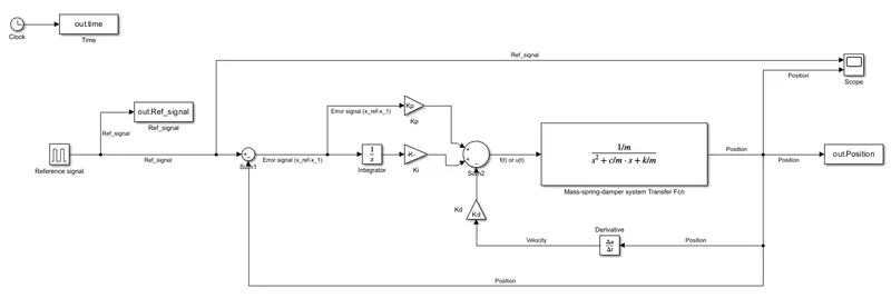
In order to generate a pulsed reference input signal of 5s width, 10s time period and amplitude of 1, a pulse generator block has been used. Inside this pulse generator block, the amplitude has been selected as 1, the period is selected as 10 s, the pulse width as 50 %, and the phase delay as 0 sec. The pulse type is time based and the simulation time is used for the generation of pulses.
The entire MSD system is represented as a Transfer function block. According to the transfer function of an MSD system we know `G(s)=(X(s))/(F(s))=(1/m)/(s^2+(c/m)s+k/m)`
The input to the MSD transfer function block or the plant is the forcing function f(t) or the control input 'u'. And the output of the plant is position or displacement.
Therefore inside the transfer function block, the numerator co-efficient is selected as [1/m], and the denominator co-efficient is selected as [1 c/m k/m], where the values of m,k, & c are obtained from running the Matlab script file as presented earlier.
To get the control signal 'u' or the forcing function f(t) which is the input to the Mass-spring-damper plant, the reference signal is first compared with the position signal using a Sum block. The sign of this Sum block is selected as +-. For proportional control this ouput is multiplied with a gain block Kp; and for integral control this output is first passed through an integrator block and then multiplied with the gain block Ki. To get the velocity signal `x_2` the position signal is fed to a derivative block. And this velocity signal is multiplied with the gain block Kd for differential control. Next all the three outputs of of the controller gain blocks are summed together using a sum block whose sign is taken as ++-. The output of this sum block is the input to the plant. The gains Kp and Kd are available from running the script file as presented above, whereas only Ki is varied manually to get a better sytem response.
Intially the value of Ki is set to a nominal value of 100, and the whole system is simulated. Next Ki is gradually varied to see the change in the response nature.
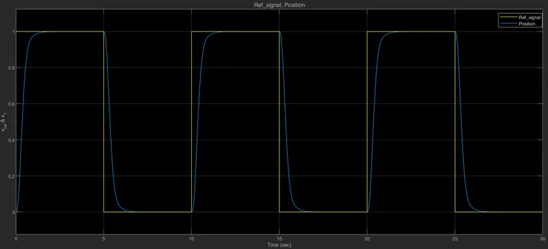
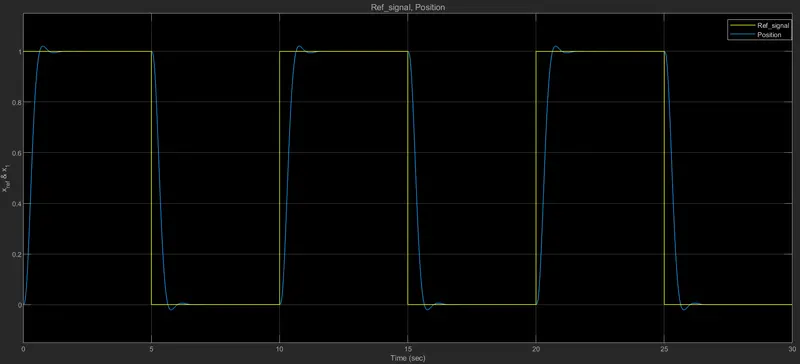
The reference input and the position output is shown with a scope.
The simulation time is taken as 30 seconds, and in the model setting the fixed step solver type is used with a step value of 0.001.
Output:
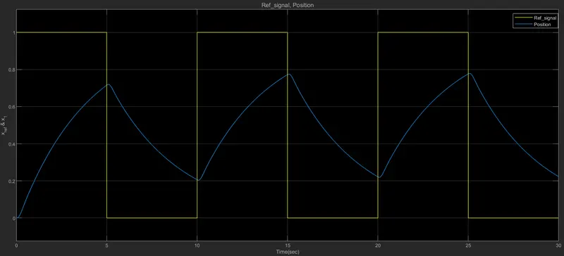
When Ki is set to 100
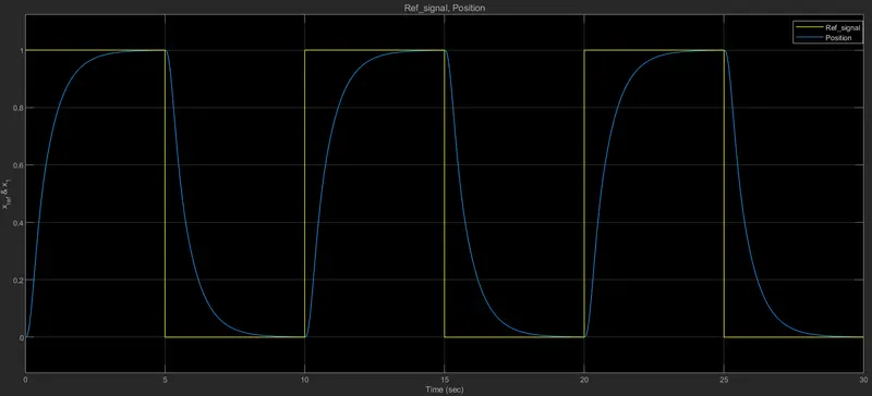
When Ki is set to 500
When Ki is set to 1000
When Ki is set to 1250
When Ki is set to 1500
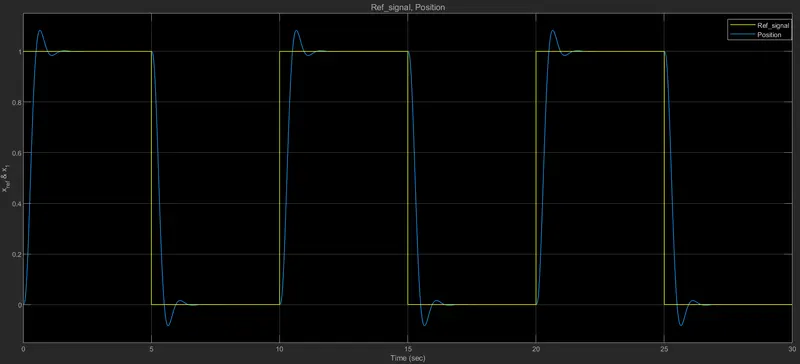
Conclusion: In this project we derived the position to forcing input transfer function of a given Mass-Spring-Damper system, analyzed its nature in terms of damping ratio and natural angular frequency of oscillation and found out that the the open loop system is overdamped in nature. Therefore in order to track a given reference position input in a faster manner, we designed a controller such that the closed loop system's response is underdamped in nature. In the simulation results, the yellow line in the scope shows the reference pulse input with a time period of 10 seconds and a pulse width of 5 seconds having an amplitude of 1 unit. The blue line shows the system's response, i.e., the position of the Mass-Spring-Damper system. From this result we can observe that as we increase the integral gain Ki, the system's response is gettng better. By increasing Ki, we are reducing the Rise time and the steady state error of the sysetm. Although there is some increase in the response overshoot and settling time. From the above plots we see that Ki=1250 gives better response than other ones, the response is fast enough and also the overshoot is less than Ki=1500 case. Therefore it can be concluded that the designed controller with an integral gain Ki=1250 gives satisfactory result, the response is fast with overshoot less than 2 %, and also the system's response tracks the refrence pulse input.