Project - Position control of mass spring damper system
Question
Obtain the transfer function of a mass spring damper system and use it in the model. Add a PID controller to adjust the
force on mass so that its position follows a reference signal.
Take m = 3.6; %kg k = 400; %N/m c = 100; %Ns/m
The reference signal is shown in the following figure.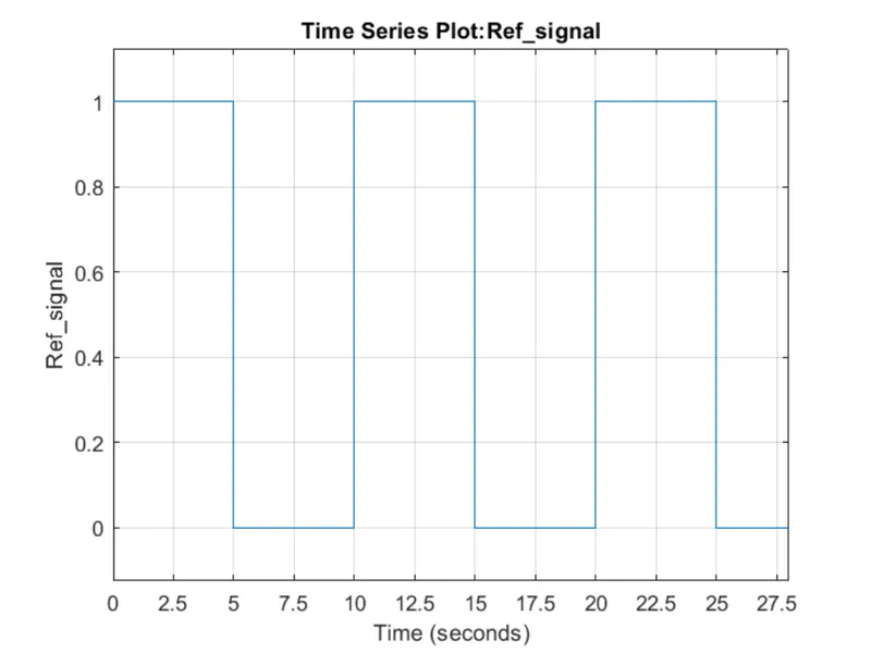
Answers
objective:
position control of the mass-spring-damper system for the mentioned reference signal:
Developing the model Position control of mass spring damper system
Obtain the transfer function of a mass spring damper system and use it in the model. Add a PID controller to adjust the
force on mass so that its position follows a reference signal.
Take m = 3.6; %kg k = 400; %N/m c = 100; %Ns/m.
We know the general equation for mass spring damper system s given by
x_dot = Ax + Bu
So the state representation of our spring mass system can be given by
x1_dot = x2 --------------------------------------(1)
x2_dot = -(k/m) + (1/m)u ----------------------------------------(2)
We are using PID controller. So it has three gains Kp,Kd and Ki
So u = [Kp(x_ref – x1) – Kdx2 + Ki inte(x_ref – x1)]
Then the equation (2) becomes
x2_dot = -(k/m) + (1/m) [Kp(x_ref – x1) – Kdx2 + Ki inte(x_ref – x1)] ------------(3)
We have to design the model for equation(3)
Where
Kp – is proportional gain
Kd – is integral gain
Ki – is integral gain
m – is mass of the spring mass system
k – is a stiffness or spring constant
x2_dot – is accelaration
x1_dot = x2 – is a velocity
x1 – is displacement
The input to the model is given by the following MATLAB script
Script codes:.
%c=2*zeta*wn
%for zeta=0.5, c=2*(0.5)*(6.2832),c=6.2832
%c=100 given on the question
m=3.6; % mass of the system
k=400.0; % spring constant
wn=sqrt(k/m);%Find out the wn value by using formula
% Angular frequency m=3.6; % mass of the system
k=400.0; % spring constant in rad/sec
fn=1; % fn=wn/(2*pi), Natural frequency in Hz
zeta=0.5; %Defining Zeta to 0.5 damping ratio
p1=-zeta*wn+wn*sqrt(zeta^2-1); % first pole of characteristic equation
p2=-zeta*wn-wn*sqrt(zeta^2-1); % second pole of the characteristic equation.
P=[p1;p2]; % P vector stores the two poles
% A and B matrices from state space representation
c=100;
A=[0 1;-k/m -c/m];
B=[0;1/m];
% Pole placement design using 'place' Command
K=place(A,B,P);
Kp = K(1); % Kp is a proportional gain
Kd = K(2); % Kd is a derivative gain
Ki=1000;
Simulink model:
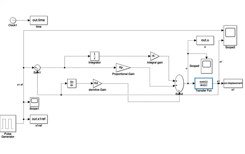
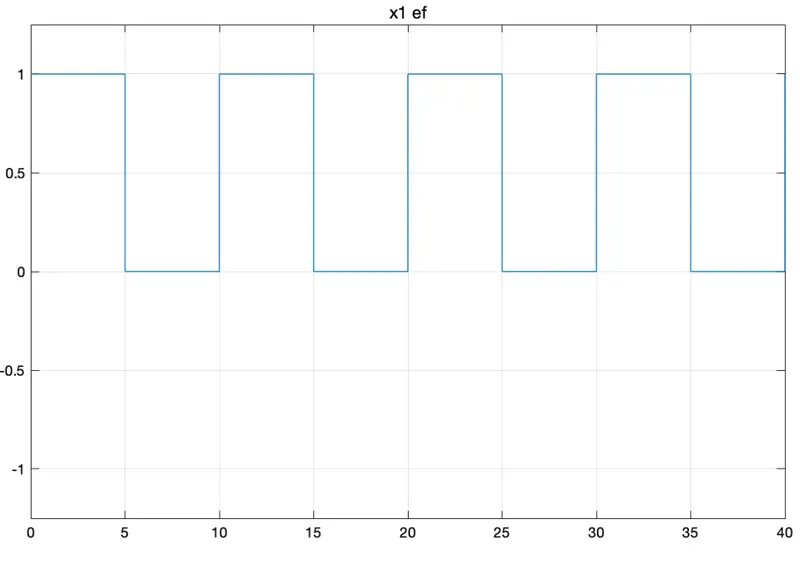
Scope images are below:
Inut x1 ref: scope:1
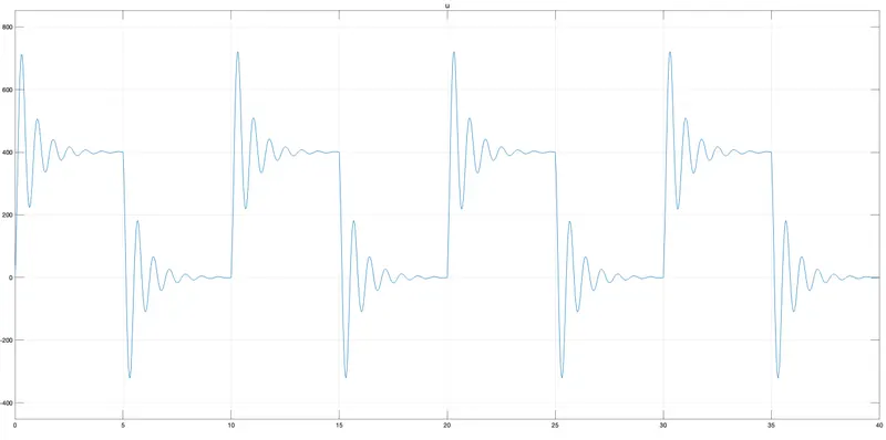
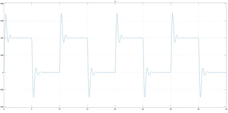
Outpit: u Scope 2
Output x1: Scope 3
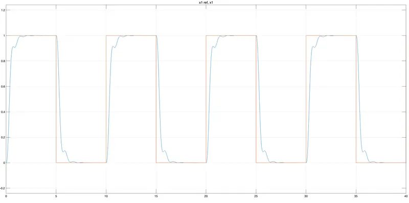
Where Ki is 1500
We have change the Ki vlue is 1500. will seee the input and output values
Inut x1 ref: scope:1
Outpit: u Scope 2
Output x1( Displacement): Scope 3
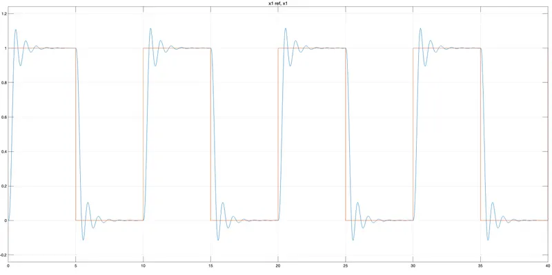
We got ourput similsr square waveform ar ki is 1500.