Challenge

Project - Position control of mass spring damper system

PID (Proportional, Integral, and Derivative) Control Design
- The general Structure of the PID controller,
  
  `u(t) = Kp*e(t) + Ki*inte(t)*dt +Kd*(de(t))/dt`
  
  where e(t) - Error between the reference input and measure output
  
  Kp, Ki, and Kd - The proportional, integral, and derivative gains.

Explanation
- The Transfer function for the spring mass damper system is X(s)/F(s)=1/ms^2+cs+k where X(s) is the displacement of the position wrt the force acting on the mass. F(s) is the force applied to the mass.
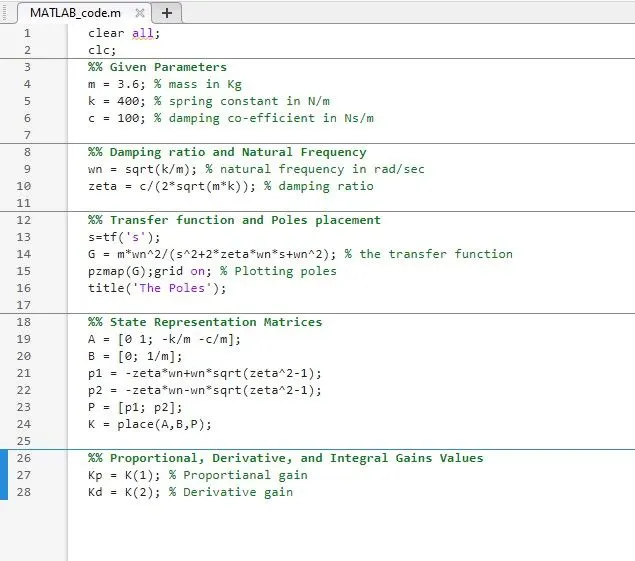
- To control the displaced position of the mass after the force acting on it, we have to use a PID controller. Here zeta value=1.3176 (Overdamping condition) is considered by using zeta value Poles(p1, p2) are calculated, and then Calculate Kp (Proportionality constant), Kd (differential constant) by using the place command. Ki (Integral Constant) value is manually modified to control the output wrt input. Here the input is a pulse-generated signal with an amplitude of 1 and a period of 10 as given.

Control Design Objectives
- Settling time <2 sec
- Overshoot < 5%
- Steady-state error < 1%

clear all;

clc;

%% Given Parameters

m = 3.6; % mass in Kg

k = 400; % spring constant in N/m

c = 100; % damping co-efficient in Ns/m

%% Damping ratio and Natural Frequency

wn = sqrt(k/m); % natural frequency in rad/sec

zeta = c/(2*sqrt(m*k)); % damping ratio

%% Transfer function and Poles placement

s=tf('s');

G = m*wn^2/(s^2+2*zeta*wn*s+wn^2); % the transfer function

pzmap(G);grid on; % Plotting poles

title('The Poles');

%% State Representation Matrices

A = [0 1; -k/m -c/m];

B = [0; 1/m];

p1 = -zeta*wn+wn*sqrt(zeta^2-1);

p2 = -zeta*wn-wn*sqrt(zeta^2-1);

P = [p1; p2];

K = place(A,B,P);

%% Proportional, Derivative, and Integral Gains Values

Kp = K(1); % Proportianal gain

Kd = K(2); % Derivative gain

Building a Model
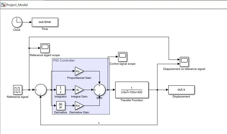
- Clock block is used to time input and save it to a variable 'out.time'.
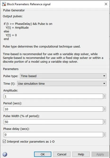
- Here the reference signal F(s) is a pulse-generated signal with an amplitude of 1 and a period of 10 as given.
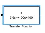
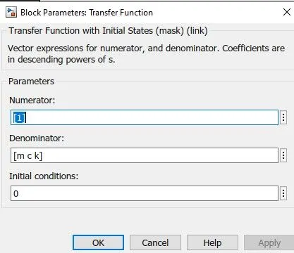
- Using the transfer function block with initial condition zero and put the transfer function in the block.
- Creating the error signal [e(t)=referance signal - x1] by using the sum block.
- Creating control signal [u(t)] by sum block with the gain blocks having values of proportional gain (Kp), and derivative gain (Kd).
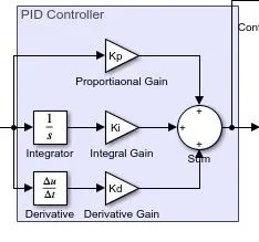
- Adding scope blocks to represent the reference signal, control signal, and displacement vs reference signal.
- Different variable name:
  - out.x - displacement
  - out.time - time
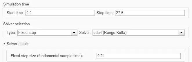
- In the model, the simulation is 0 to 27.5 sec., the solver type is the fixed type with step size 0.01 and the solver is ode4(Runga-Kutta).

Analysis
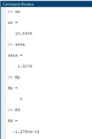
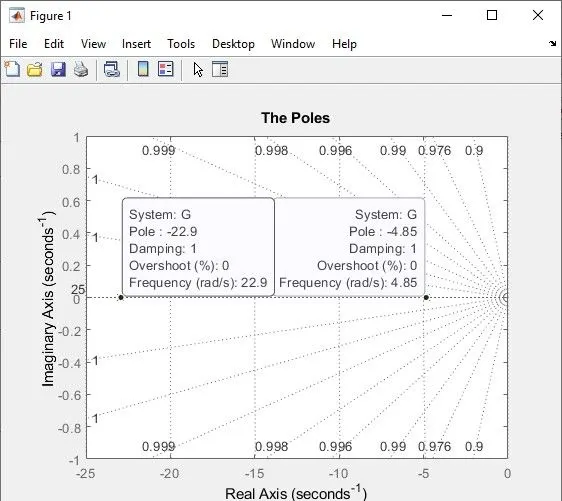
- Hereafter running the MATLAb script, we have Kp = 0 and Kd = -1.2790e-14. And the poles of the system are negative real unequal parts and there are located in the left-hand plane which concludes that the system is an overdamped and stable system.
- With the transient response moving slowly toward the steady state or the equilibrium point with some oscillation.
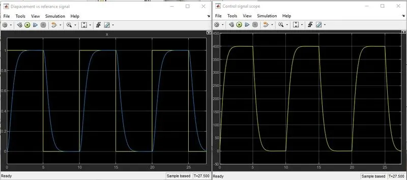
- Case 1, Ki = 500
  - Settle-time is approximately 2.5 sec.
  - Overshoot is 0%.
  - Steady-state error is less than 1%.
  - Rise time is approximately 2.5 sec.
- Case 2, Ki = 1000
  - Settle-time is approximately 2.5 sec.
  - Overshoot is more than 5%.
  - Steady-state error is less than 1%.
  - The rise time is approximately 1.5 sec.
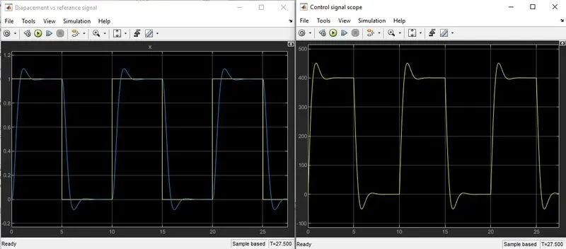
- Case 3, Ki = 1500
  - Settle-time is approximately 2.5 sec.
  - Overshoot is more than 5%.
  - Steady-state error is less than 1%.
  - Rise time is approximately 1 sec.
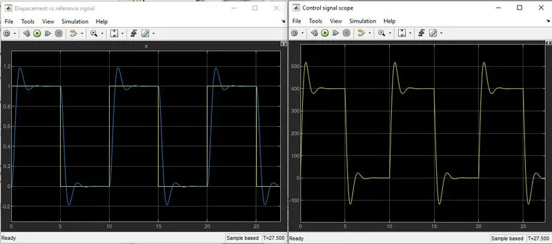
Conclusion
- For achieving the control design objective we have to change the values of the Kp and Kd which is almost equal to zero.
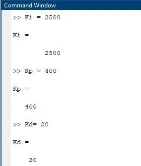
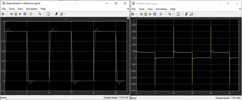
- Consider the values of Kp is 400, Kd = 20, and Ki is 2500.

Ship work like this
in your own course.