Project - Data Handling and Interpolation
Aim: Interpolation and Data handling.
Objective:
Perform the interpolation in the range of -17.3:0.1:0.9. Generate the interactive plot for the
interpolated data and store them in a text file.
Introduction:
Interpolation is a technique for adding new data points within a range of a set of known
data points.We can use interpolation to fill-in missing data, smooth existing data, make
predictions, and more. Interpolation in MATLAB ® is divided into techniques for data points on a grid
and scattered data points.
Use of the interp1 function to determine and plot interpolated data for given data.
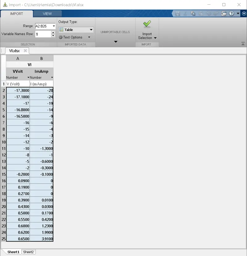
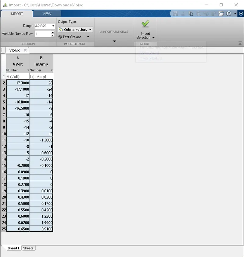
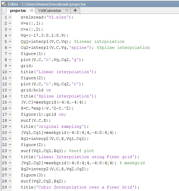
1. Using the xlsread function read the data and store it in the variable called x.
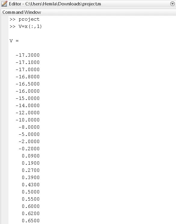
2. from that extracted the first column which is voltage data and stored as variable V
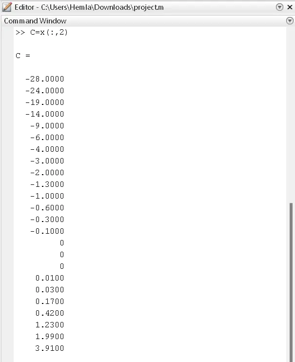
3. Also extracted the second column which is current data stored as variable C.
4. Perform the interpolation in the range of -17.3:0.1:0.9 store it in the variable called Vq.
5. Then we interpolated the curve by adding some range of data in function interp1 Cq1.
6. Smooth the data by spline interpolation method Cq2.
7. Then plotted various curve such as:
1.Linear intrpolation,
2. Spline interpolation,
3. Original sampling,
4. Linear Interpolation using Finer grid,
5. Cubic Interpolation over a Finer Grid.
8. Here we have used meshgrid function.
9. Grid: The grid on Matlab is the lines that are meant to separate the rows and columns which are
used for computational purposes.
About Meshgrid:
MeshGrid is one of the most important functions in Matlab which is mainly used while
creating various plots in Matlab like Surface, polar, and Mesh plots. They are used in maps
for various geographical locations, designing and Computational Fluid Dynamics.
Imported data:
Script:
x=xlsread('VI.xlsx');
V=x(:,1);
C=x(:,2);
Vq=(-17.3:0.1:0.9);
Cq1=interp1(V,C,Vq); %Linear intrpolation
Cq2=interp1(V,C,Vq,'spline'); %Spline interpolation
figure(1);
plot(V,C,'o',Vq,Cq2,'g');
grid;
title('Linear interpolation');
figure(2);
plot(V,C,'o',Vq,Cq2,'r');
grid;hold on
title('Spline interpolation');
[V,C]=meshgrid(-4:4,-4:4);
Z=C.*exp(-V.^2-C.^2);
figure(1);grid on;
surf(V,C,Z);
title('Original sampling');
[Vq1,Cq1]=meshgrid(-4:0:4:4,-4:0:4:4);
Zq1=interp2(V,C,Z,Vq1,Cq1);
figure(2);
surf(Vq1,Cq1,Zq1); %surf plot
title('Linear Interpolation using Finer grid');
[Vq2,Cq2]=meshgrid(-4:0:4:4,-4:0:4:4); % meshgrid
Zq2=interp2(V,C,Z,Vq2,Cq2);
figure(3);
surf(Vq2,Cq2,Zq2);
title('Cubic Interpolation over a Finer Grid');
Output:
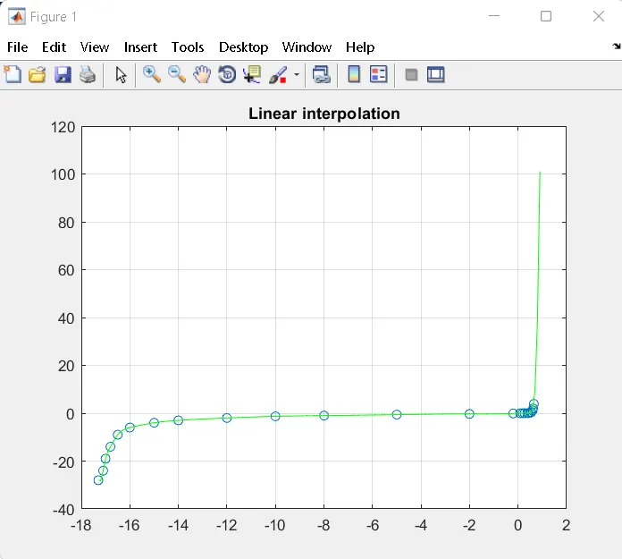
1. Linear interpolation:-
The function to perform linear interpolation, MATLAB provides the interp1() function.
Here, a sample point is a set of data points, which could be an array or a vector. The value of the
unknown function on sample points is also a set that has the same size/length as the sample points.
The third argument could be a set or a single value that has the data at which interpolation is to be
performed. The fourth argument is optional, and it tells MATLAB which method of interpolation is to
be used. By default, it is set to linear thus, we would not change it.
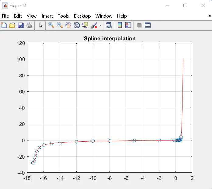
2. Spline interpolation:-
s = spline (V, C, Vq) returns a vector of interpolated values s corresponding to the query points in
Vq. The values of s are determined by cubic spline interpolation of V and C. example. pp = spline (V,
C) returns a piecewise polynomial structure for use by ppval and the spline utility unmkpp.
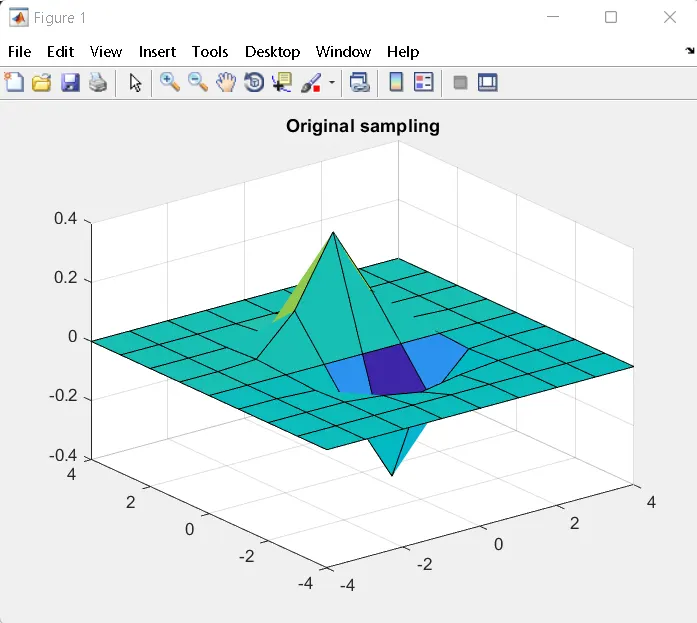
3. Original Sampling:-
4. Linear Interpolation using finer grid:-
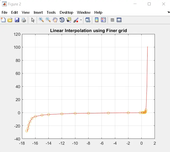
From the graph it is concluded the interpolated values at the query point which is based on the
values of grid points in each dimension defined. There are certain limitations of this method like 2
points are at least required to use Linear Interpolation.
5. Cubic interpolation over a Finer grid:-
Interpolate over a finer grid using ntimes=1. Vq = interpn (V, 'cubic'); mesh (Vq); Evaluate Outside
Domain of 3-D Function Create the grid vectors, V1, V2, and V3. These vectors define the points
associated with the values in V.
Results in Command window:
Interpolated data stored in .txt file:
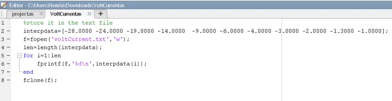
1.For storing the interpolated data, we first open the file in write mode using fopen function pointer
called f.
2. Using the for loop we printed the data in the VoltCurrent.txt file.
3. And closed the file.
Script:
% store it in the text file
interpdata=[-28.0000 -24.0000 -19.0000 -14.0000 -9.0000 -6.0000 -4.0000 -3.0000 -2.0000
-1.3000 -1.0000];
f=fopen('voltCurrent.txt','w');
len=length(interpdata);
for i=1:len
fprintf(f,'%d\n',interpdata(i));
end
fclose(f);
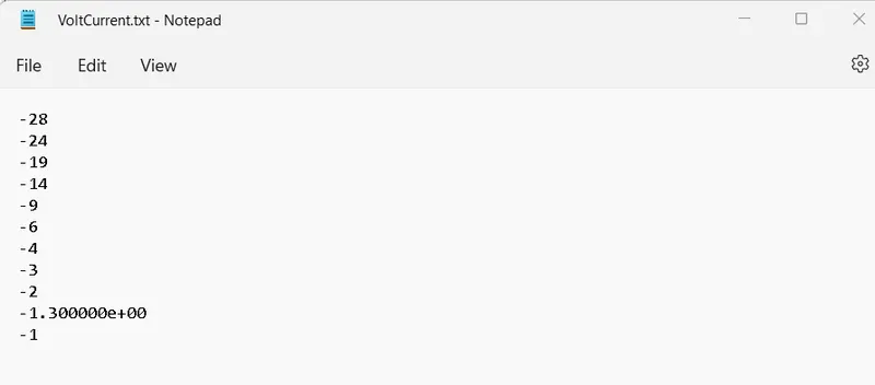
Result of a .txt file:
Conclusion:
In this project, we have succefully perform the interpolation in the range of -17.3:0.1:0.9. And also
generate the interactive plot for the interpolated data and store them in a text file.
Link:
https://drive.google.com/file/d/1tQ4TeoiZzj_jplItGO9cfVEXc_5i-RE-/view?usp=sharing
https://drive.google.com/file/d/12avhOhhsTvnWsSM_13NAs8jd9Er2fTFp/view?usp=sharing
https://drive.google.com/file/d/108PLWvtv5-7vuFUDK-HpICpR_UxWg8U5/view?usp=sharing