Project

PROJECT

AIM: To study and analyse the BAJA All- terrain vechicle (ATV) model using simulink and prepare a technical report of simulation of ATV under different conditions.

OBJECTIVE: Prepare technical report explaining the model properties and comments on the results. 

DESCRIPTION:

 ALL-TERRAIN VECHICLE(ATV)

     An All-terrain vechicle, also known as Quad(cycle), Light utility vechicle, as defined  by the American National Standards Institute(ANSI), is a vechicle that travels on low-pressure tyres, with a seat that is straddled by the operator, along with the handlebars for steering control. It is f=designed to handle a wider variety of terrain than most other vechicles. ATVs offer excellent off-road capabilities and can carry heavy equipment over over long distances and narrow access points.

                                                                        

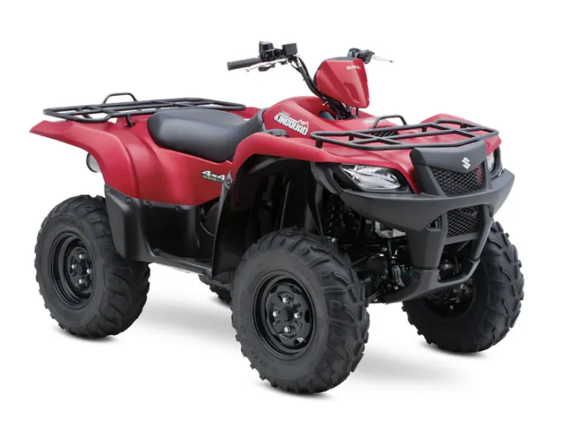
                                                                 Fig 1.1  All Terrain-Vehicle (AVT)

 COMPONENTS OF ATV   

   The components used in ATVs are;

• Vechicle body
• Suspension
• Tire
• Engine
• Continiously variable transmission(CVT)

                                                    

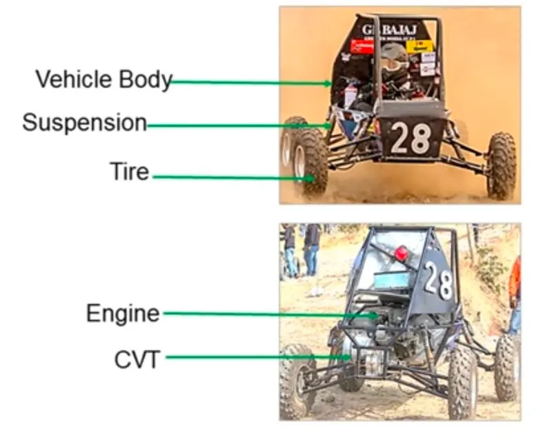
                                                              Fig 1.2

CONTINIOUSLY VARIABLE TRANSMISSION

A continiuosly variable transmission is an automatic transmission that can change semlessly throug a continious range of gear ratios. This contrasts with other transmissons that provides a limited number of gear ratios in fixed steps. The flexibility of a CVT with suitable control may allow the engine to operate at a constant RPM while the vechicle moves at varying speeds. CVT uses two pullys having variable diameters that help the transmission achieve infinite gear ratios. The figure below (fig 1.3) consists of primary pully, variator, seconndary pully and a belt. When variator , which is connected to the primary pully moves outwards, then vaiator of secondary pully will move inwards such that radius of primary pully is less than the radius of secondary pully which leads to speed reduction and when variator which is connected to the primary pully move inwards then variator of secondary pully will move outwards such that radius primary pully is more than the radius of secondary pully which leads to overdrive. 

                                              

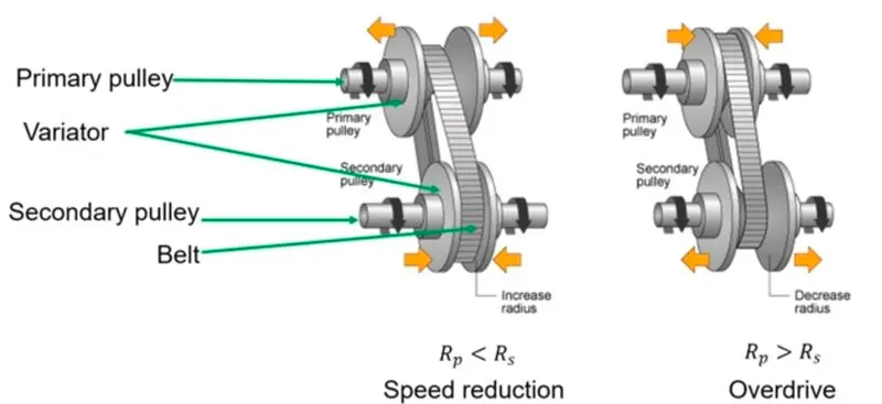
                                                Fig 1.3 Continiously Variable Transmission(CVT)

1. BAJA ATV MODEL

                          

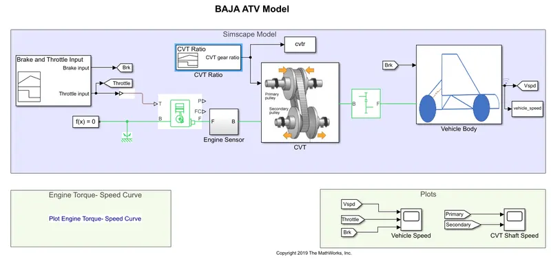
                          Fig 1.4 BAJA ATV Model

The input signal is provided using signal builder block in which brake input is provided as 0 and throttle input is provided as 0.3 upto 20s and varied to 1 for remaining seconds.

                        

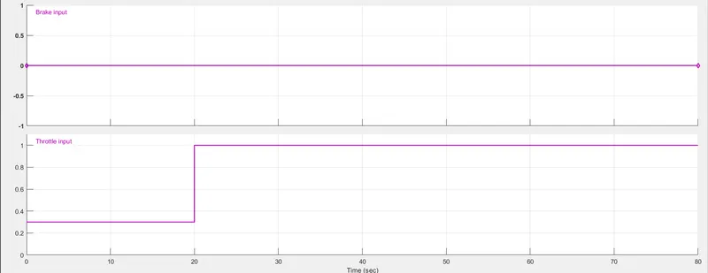
                        Fig 1.5

• GENERIC ENGINE

 The engine uses a programmed relationship between speed and torque, modulated by throttle signal. The throttle input signal T lies between 0 and1 and specifies the torque demanded from the engine as a fraction of the maximum posiible torque. Connections F and B are mechanical rotational conserving ports assosciated with the engine crankshaft and engine block, respectively. Connections P and FC are physical signal ouput ports through which engine power and fuel consumption rate are reported.

                                                 

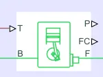
                                                 Fig 1.6 Generic engine

• CVT BLOCKSET       

                            

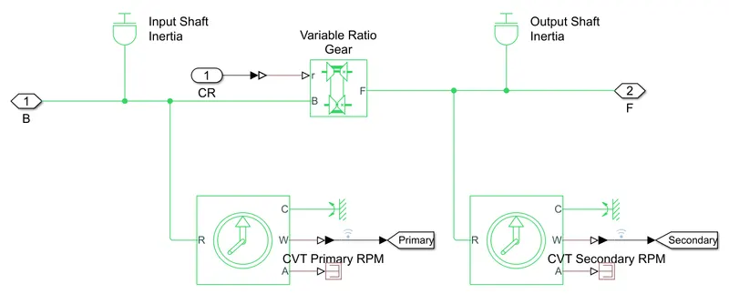
                                Fig 1.7

 Input shafts represents the primary pully and output shafts represents the secondary pully and mechanical rotational sensor is connected to input and ouput shafts and variable ratio gear represents a variable ratio gearbox such as implemented  by mechanical belt CVT, electric, or hydraulic  transmissions. The physical input 'r' defines the ratio of input to output angular shaft  velocities. Connections B and F are mechanical rotational conserving points.

• VECHICLE BODY

Represents a two-axle vehicle body in longitudinal motion. The block accounts for body mass, aerodynamic drag, road incline, and weight distribution between axles due to acceleration and road profile. The vehicle can have same or a different number of wheels on axle. Optionally include pitch and suspension dynamics or additional variable mass and inertia. The vehicle does not move vertically relative to the ground. The below fig consists of four wheels at the rear and the other two at the front. The rear wheel is connected with a double shoe break which represents a break arranged as two pivoted right shoes symmetrically installws inside or outside a drum and operated by one actuator. The actuator force causes the shoe to exert friction torque on ashift connected to the drum.

                                                

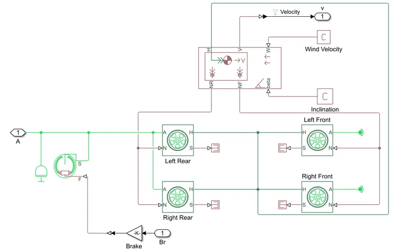
                                          Fig 1.8

• CVT GEAR RATIO INPUT

                                 

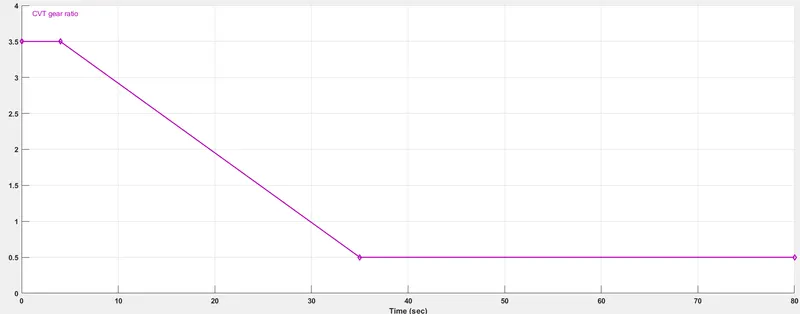
                                 Fig 1.9

• TORQUE VS ENGINE SPEED INPUT

                                

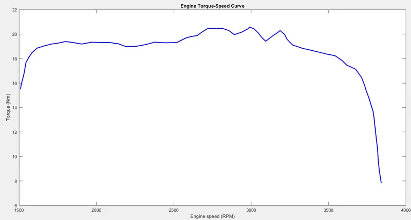
                                Fig 1.10

RESULTS

  a.  VECHICLE SPEED

                      

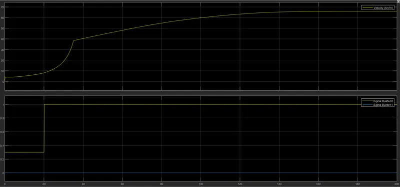
                               Fig 1.11

 The above plot shows that when throttle is at 0.3 for 20s, the speed of vechicle increases correspondisly and at full throttle the vechicle speed is jumped nearly to speed of 40km/h and then increases propertionally.

  b.  CVT SHAFT SPEED 

                             

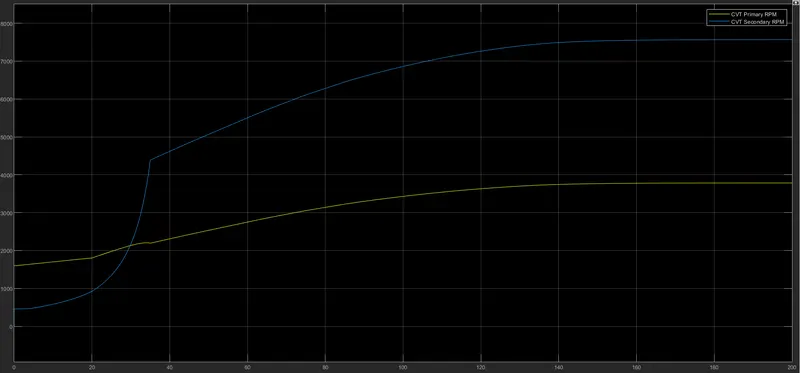
                             Fig 1,12

    From the above plot, it can be obseved that CVT secondary RPM plot and velocity of the vechicle from the previous plot behaves same because the secondary pully is connected to the vechicle output.

2. BAJA ATV MODEL WITH LOOK UP TABLE

                           

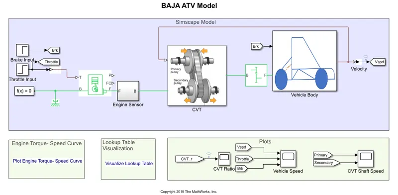
                                           Fig 2.1

The above model of BAJA ATV with CVT along with the look up table is similar to the previous model. Only difference is that the CVT ratio is provided in look up table.

• LOOKUP TABLE

  A lookup table is an array of data that maps input values to output values, thereby approximating a mathematical function. Given a set of input values, a lookup operation retrives the corresponding output values from the table. If the lookup table does not explicitly define the input values, simulink can estimate an output value using interpolation, extrapolation or rounding. 

                                

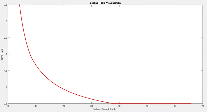
                                         Fig 2.2

• CVT BLOCK

                               

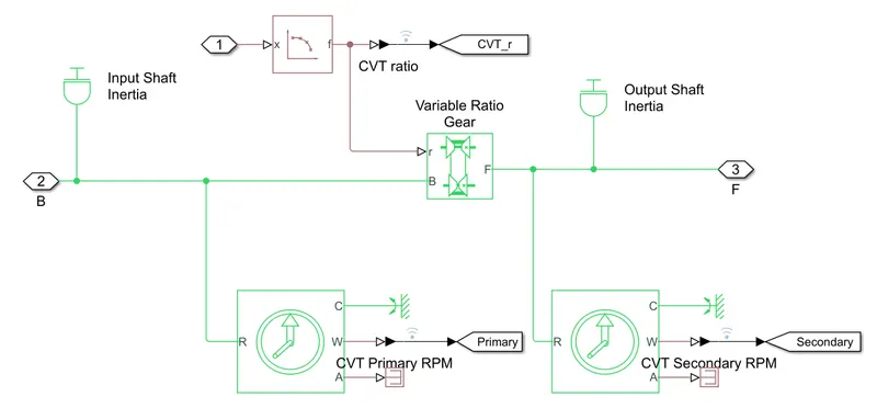
                                 Fig 2.3

Input shaft represents the primary pully and output shafts represents the secondary pully and mechanical rotational sensor is connected to input and output shafts and variable ratio gear represents a variable rato gearbox such as implemented by mechanical belt CVT, electric or hydraulic transmissions. The physical signal r defines the ratio of input to output angular shaft velocities. Connections B and F are mechanical rotational conserving ports.

RESULTS

1.  CVT RATIO

                

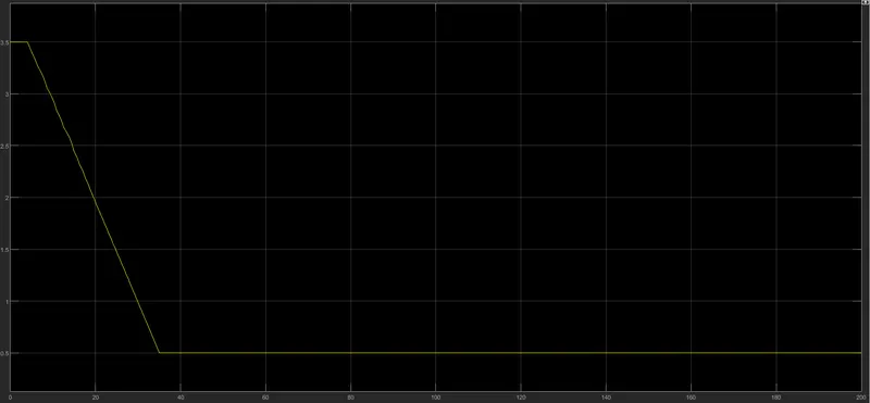
                Fig 2.4

The above data is obtained from lookup table.

    b.  VECHICLE SPEED

                

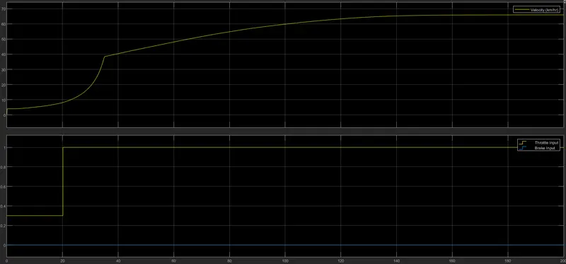
                Fig 2.5

 The above plot shows that when throttle is at 0.3 for 20 s, the speed of vechicle increases correspondingly and at 1( at full throttle), the vechicle speed is jumped nearly upto 40km/h and then increases proportionally and the result remain same as the input parameter reman same.

    c.  CVT SHAFT SPEED

               

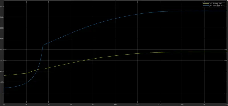
               Fig 2.6

From the above plot, it can be obseved that CVT secondary RPM plot and velocity of the vechicle from the previous plot behaves same because the secondary pully is connected to the vechicle output.

3. BAJA ATV MODEL WITH DASHBOARD

                   

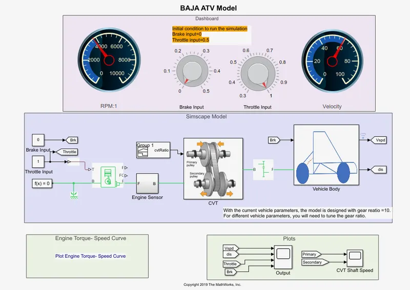
                   Fig 3.1

RESULTS

  a.  VEHICLE SPEED

                   

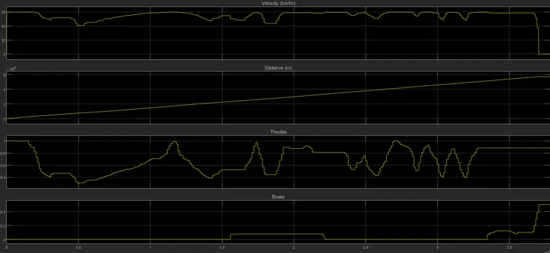
                   Fig 3.2

The above plot shows the variation of throttle as provided in the dashboard and corresponding velocity and distance tavelled by the vehicle.

  b.  CVT SHAFT SPEED

                  

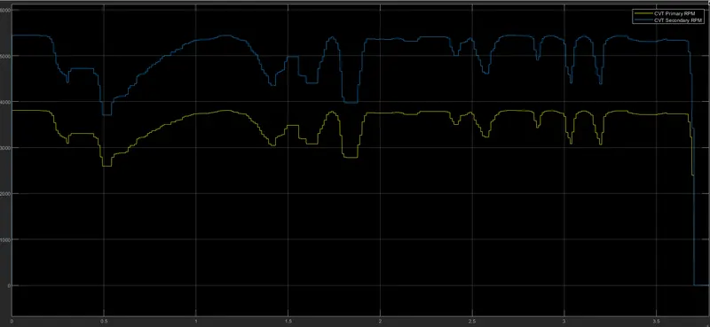
                  Fig 3.3

From the above plot, it can be obseved that CVT secondary RPM plot and velocity of the vechicle from the previous plot behaves same because the secondary pully is connected to the vechicle output.

4. BAJA ATV MODEL WITH DASHBOARD AND LOOKUP TABLE

                           

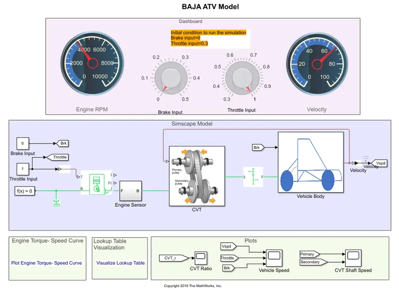
                              Fig 4.1

The above model is similar to that of the previous one with lookup table and the only difference is that the input signal provided through knob in the dashboard, and the corresponding velocity of the vechicle is observed.

• LOOKUP TABLE

                             

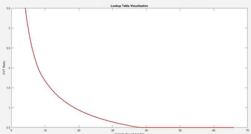
                             Fig 4.2

RESULTS

  a.  VEHICLE SPEED

                             

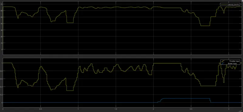
                             Fig 4.3

  The above plot we can see that velocity follows the same path as input which is throttle input and breake point.

  b.  CVT SHAFT SPEED

                            

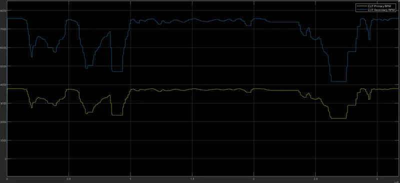
                            Fig 4.4

From the above plot, it can be obseved that CVT secondary RPM plot and velocity of the vechicle from the previous plot behaves same because the secondary pully is connected to the vechicle output.

CONCLUSION 

   We have succesfully stimulated the 4 different model of BAJA ATV with CTV and satisfactory results are obtained by variying the input data.