Project
Aim- Carry out a system-level simulation of an all-terrain vehicle using simulink.
Download the model from the given link:
https://www.mathworks.com/matlabcentral/fileexchange/70576-baja-all-terrain-vehicle-atv-model
Prepare a technical report explaining the model properties & comments on the results.
Theory-An all-terrain vehicle (ATV) is defined as a motorized off-road vehicle designed to travel on four low-pressure or non-pneumatic tires, having a seat designed to be straddled by the operator and handlebars for steering control. ATVs are subdivided into two types as designated by the manufacturer.
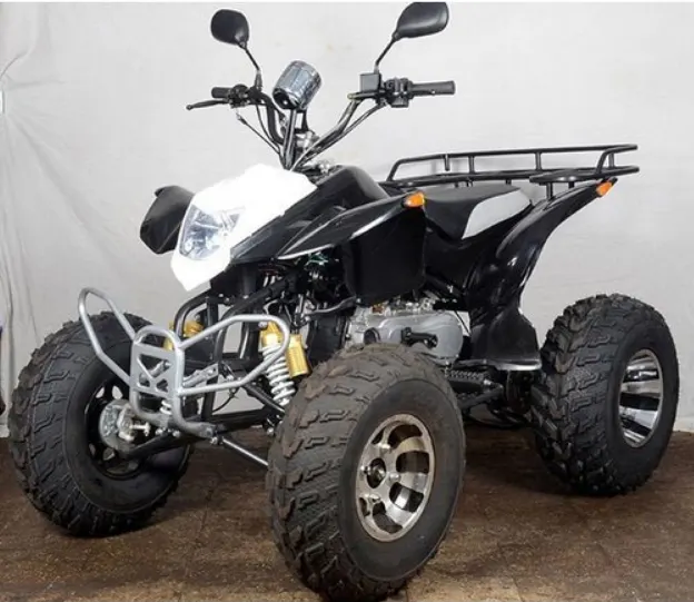
Type-I: ATVs are intended by the manufacturer for use by a single operator and no passenger.
Type-II: ATVs are intended by the manufacturer for use by an operator and a passenger, and are equipped with a designated seating position behind the operator.
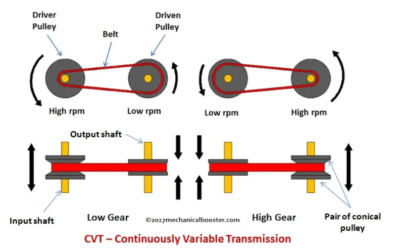
CVT-A continuously variable transmission system is a type of automatic transmission in which an arrangement of pulleys and belts made it possible for a drive to achieve n-number of continuous gear ratios within a range (depends on the design).
A continuously variable transmission in a vehicle senses the accelerator input with engine load and get shifted to the desired speed or torque gear ratio automatically, in other words we can say that a cvt transmission is one of the simplest types of automatic transmission that provides continuous uninterrupted power within a specified range of speed and torque ratios.
TYPES OF MODEL under study:-
1. BAJA ATV model without Dashboard(cvtModel)
2. BAJA ATV model with Dashboard(cvtmodel_dashboard)
3. BAJA ATV model – Mapped Lookup Table without Dashboard(cvtModel_mapped)
4. BAJA ATV model – Mapped Lookup Table with Dashboard(cvtModel_dashboard_mapped)
- BAJA ATV model without Dashboard(cvtModel)-
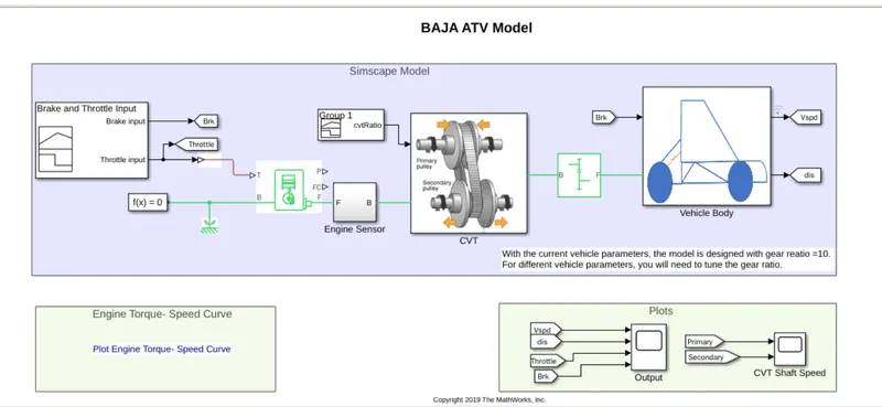
Blocks Used-
Signal Builder-The Signal Builder block allows you to create interchangeable groups of piecewise linear signal sources and use them in a model.
Goto block-The Goto block passes its input to its corresponding From blocks.
Solver configuration-The Solver Configuration block specifies the solver parameters that your model needs before you can begin simulation.
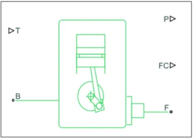
Generic engine-The Solver Configuration block specifies the solver parameters that your model needs before you can begin simulation.
Ports:
1. B - Rotational Conserving Port representing the Engine Block(should be connected to rotational motion reference)
2. F - Rotational Conserving Port representing the Engine Crankshaft
3. T- Physical signal input port :specifying the normalized engine throttle level
4.P - Physical signal output port: reporting the instantaneous engine power, in W
5. FC - Physical signal output port: reporting the fuel consumption rate, in kg/s
Mechanical Rotational Reference block- it represents a reference point, or frame, for all mechanical rotational ports. All rotational ports that are rigidly clamped to the frame (ground) must be connected to a Mechanical Rotational Reference block.
Simple Gear-The Simple Gear block represents a gearbox that constrains the connected driveline axes of the base gear, B, and the follower gear, F, to corotate with a fixed ratio that you specify
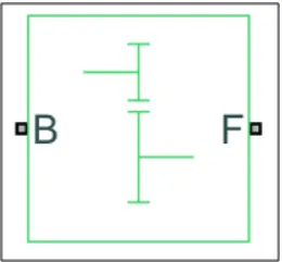
Ports: B - Base: Rotational mechanical conserving port associated with the base, or input, shaft.
F – Follower: Rotational mechanical conserving port associated with the follower, or output, shaft.
From-The From block accepts a signal from a corresponding Goto block, then passes it as output.
Variable Ratio Transmission block- The Variable Ratio Transmission block represents a gearbox that dynamically transfers motion and torque between the two connected driveshaft axes, base and follower. Ignoring the dynamics of transmission compliance, the driveshafts are constrained to corotate with a Variable Gear Ratio control that you control. You can choose whether the follower axis rotates in the same or opposite direction as the base axis. If they rotate in the same direction, wf and we have the same sign. If they rotate in opposite directions, wi and wg have opposite signs.
Transmission compliance introduces internal time delay between the axis motions. Therefore, unlike a gear, a variable transmission does not act as a kinematic constraint. You can also control torque loss caused by transmission and viscous losses.
Ports: 1. B - Base Pulley or Drive Pulley
2.F - Follower Pulley or Driven Pulley
3.r - Variable Transmission Ratio (Input)
Vehicle Body block-
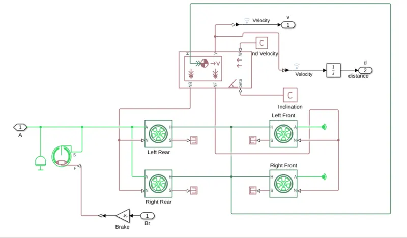
The Vehicle Body block represents a two-axle vehicle body in longitudinal motion. The vehicle can have the same or a different number of wheels on each axle. For example, two wheels on the front axle and one wheel on the rear axle. The vehicle wheels are assumed identical in size. The vehicle can also have a center of gravity (CG) that is at or below the plane of travel. The block accounts for body mass, aerodynamic drag, road incline, and weight distribution between axles due to acceleration and road profile. Optionally include pitch and suspension dynamics. The vehicle does not move vertically relative to the ground. The block has an option to include an externally-defined mass and an externally-defined inertia. The mass, inertia, and center of gravity of the vehicle body can vary over the course of simulation in response to system changes.
Limitations: The Vehicle Body block lets you model only longitudinal dynamics, parallel to the ground and oriented along the direction of motion. The vehicle is assumed to be in pitch and normal equilibrium. The block does not model pitch or vertical movement. As such, the equations assume that the wheels never lose contact. This constraint can result in negative normal forces.
Input ports:
1. Beta - Road Incline Angle (rad):physical signal input port for road incline angle
2. W – Head Wind Speed (m/s):physical signal input port for road incline angle
3. CG-center of gravity(m):physical signal input port of externally defined mass relative to the cg of vehicle(only available with externally defined additional mass is set to on)
M-mass(kg):physical signal input port for mass of the externally defined mass(only available with externally defined additional mass is set to on)
J-Externally defined moment of inertia (in kg*m^2):physical signal input port of the externally defined mass
Output ports:
1. NR - Rear Axle Normal Force (N): physical signal output port for the rear axle which is considered positive acting downward
2. NF – Front Axle Normal Force (N):physical signal output port for the front axle which is considered positive acting downward
3. V - Longitudinal Velocity (m/s):physical output signal of vehicle velocity
Conserving ports:
H - Horizontal Motion: conserving port related to the horizontal motion of vehicle body(tyres should be connected to this port)
CVT SUBSYSTEM-
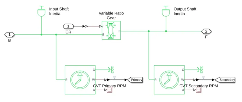
Inertia-
Input shaft inertia
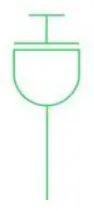
The Inertia block represents an ideal mechanical translational inertia that is described with the following equation:
T=Jdωdt
where:
-
T is inertia torque.
-
J is inertia.
-
ω is angular velocity.
-
t is time.
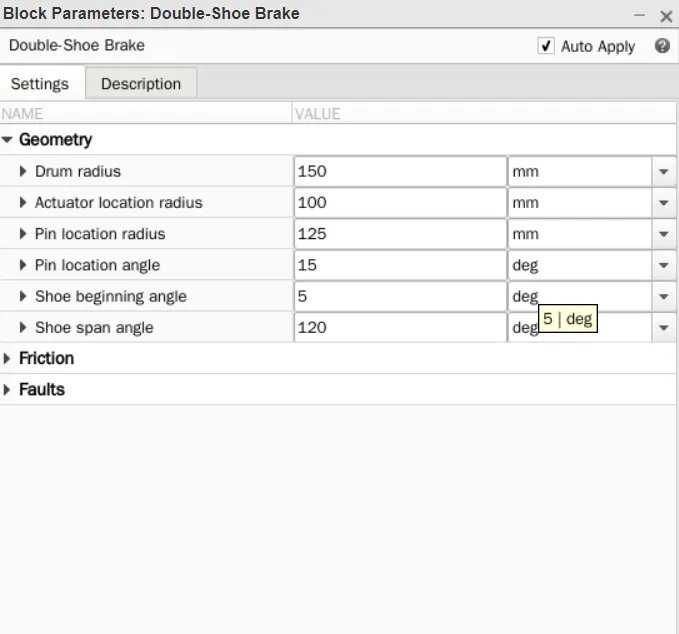
Double shoe brake-
The Double-Shoe Brake block represents a frictional brake with two pivoted rigid shoes that press against a rotating drum to produce a braking action. The rigid shoes sit inside or outside the rotating drum in a diametrically opposed configuration. A positive actuating force causes the rigid shoes to press against the rotating drum. Viscous and contact friction between the drum and the rigid shoe surfaces cause the rotating drum to decelerate.
Double-shoe brakes provide high braking torque with small actuator deflections in applications that include motor vehicles and some heavy machinery. The model employs a simple parameterization with readily accessible brake geometry and friction parameters.
You can also enable faulting. When faulting occurs, the belt will exert a user-specified force. Faults can occur at a specified time or due to an external trigger at port T
Tire-
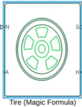
it represents the longitudinal behavior of a highway tire characterized by the tire Magic Formula. The block is built from Tire-Road Interaction (Magic Formula) and Simscape Foundation Library Wheel and Axle blocks. Optionally, the effects of tire inertia, stiffness, and damping can be included. Connection A is the mechanical rotational conserving port for the wheel axle. Connection H is the mechanical translational conserving port for the wheel hub through which the thrust developed by the tire is applied to the vehicle. Connection N is a physical signal input port that applies the normal force acting on the tire. The force is considered positive if it acts downwards. Connection S is a physical signal output port that reports the tire slip. Optionally expose physical signal port M by setting Parameterize by to Physical signal Magic Formula coefficients. Physical signal port Maccepts a four-element vector corresponding to the B, C, D, and E Magic Formula coefficients.
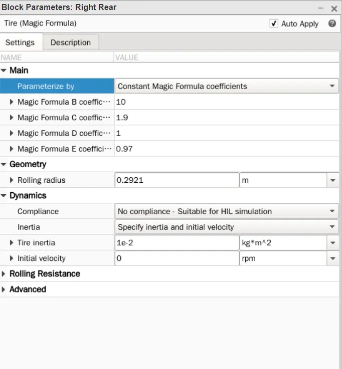
Parameters (common for all tires) are:
Engine sensor-
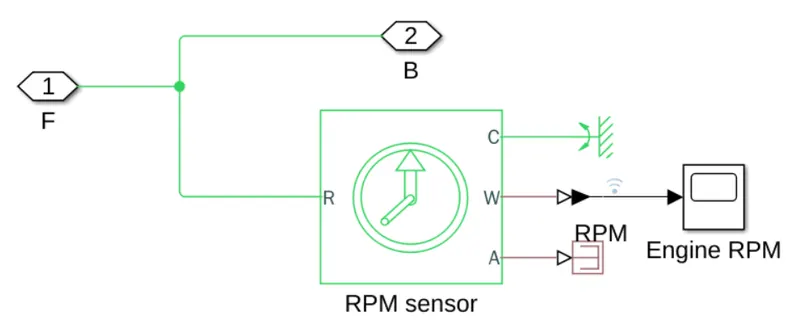
Ideal mechanical rotational motion sensor-
The block represents an ideal mechanical rotational motion sensor, that is, a device that converts an across variable measured between two mechanical rotational nodes into a control signal proportional to angular velocity or angle. The sensor is ideal since it does not account for inertia, friction, delays, energy consumption, and so on. Connections R and C are mechanical rotational conserving ports and connections W and A are physical signal output ports for velocity and angular displacement, respectively.
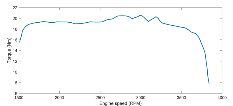
Speed-Torque characteristics-
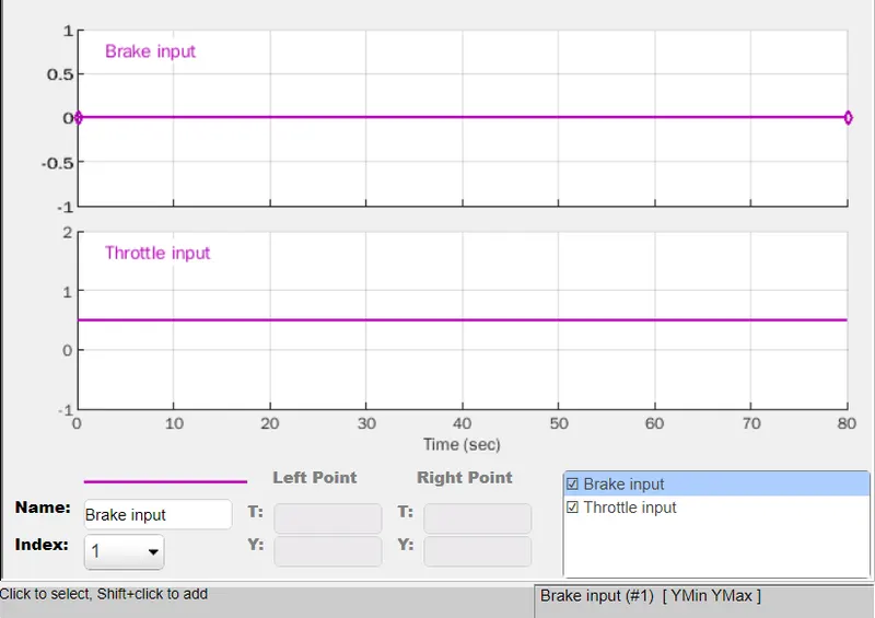
Break and Throttle input-
Brake input is constant i.e. zero throughout the time of 80 sec. Throttle input is 0.3 for first 20 sec, accelerates to 1 at the same and remains constant throughout the remaining time till 80 sec
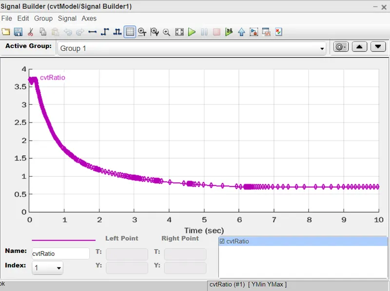
CVT ratio-
Output weaveform-
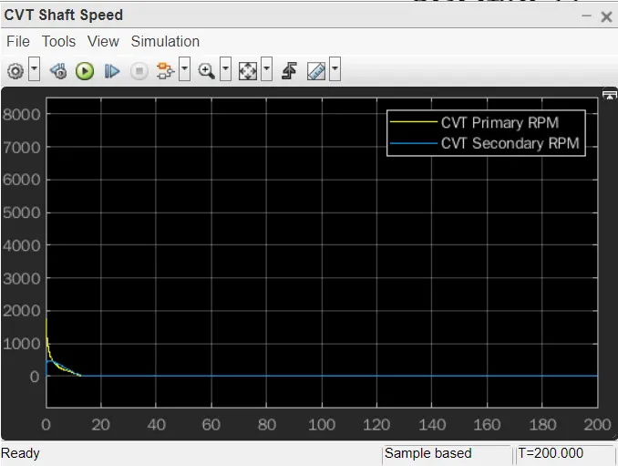
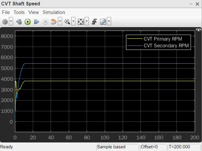
CVT shaft speed-
2. BAJA ATV model with Dashboard(cvtmodel_dashboard)-
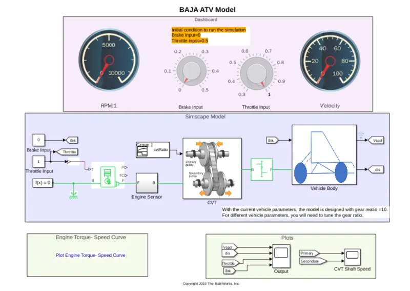
The parts and subsystem used in this model are same as above model.
Dashboard-
It is a control panel which is located in front of the vehicles driver to display the controls, speed and gear for the operation of vehicle.
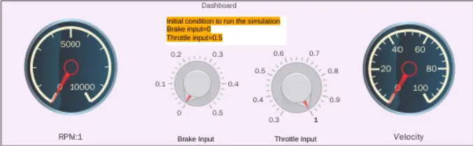
this dashboard is used to control the brake and throttle.
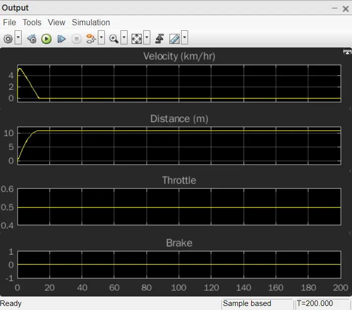
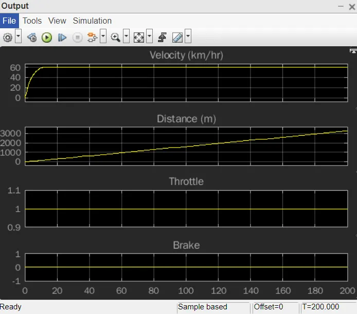
Output Waveform-
For running model 200sec-
CVT Shaft speed-
3. BAJA ATV model – Mapped Lookup Table without Dashboard(cvtModel_mapped)-
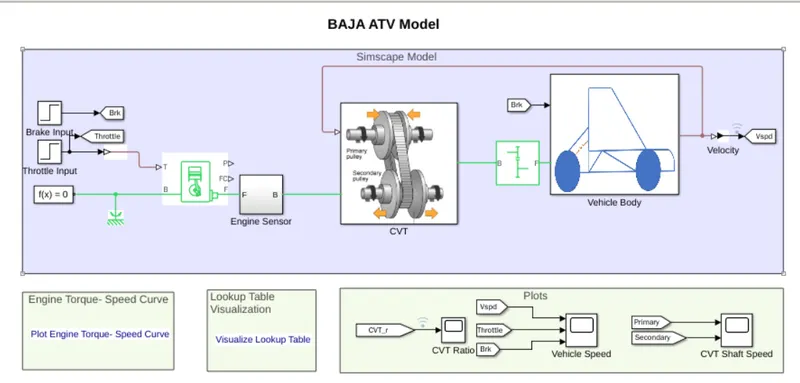
In this we have used feedback system.
4. BAJA ATV model – Mapped Lookup Table with Dashboard(cvtModel_dashboard_mapped)-
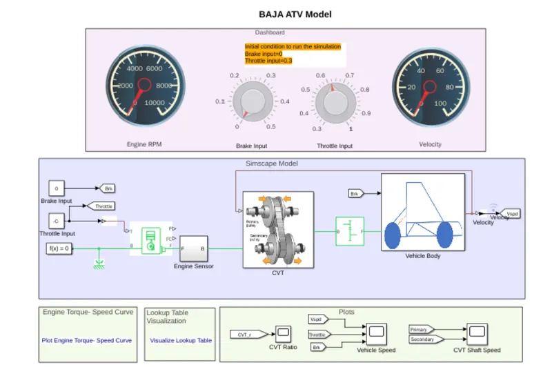
In this we have used feedback system.
Conclusion:
- Velocity, CVT Shaft Speed and Engine Speed are directly proportional to the Throttle input and inversely proportional to the Brake input.
- By increasing in braking value, the speed of vehicle decreases. while, increasing the throttle leads to increased vehicle velocity.
- CVT Primary speed is greater than CVT Secondary speed as they are directly proportional to their shaft diameter.
- The variation in vehicle velocity can be observed with change in throttle and brake inputs.