Project

ALL TERRAIN VEHICLE SIMULINK PROJECT

Aim of Project:

TO study and analyze All Terrain Vehicle(ATV) model using Simulink compare with different models.

Objective:

• Upload the supporting results as images or by any other means
• Write a detailed report
• Report attached as an image will lead to zero marks
• plagiarism is not tolerated
• upload Simulink files if needed through the google drive, any external links will not be accepted

Type of Model Studied:

• Baja ATV model without dashboard(cvt_Model)
• Baja ATV model Data Extraction(cvtModel_Data)
• Baja ATV model-Map Lookup table with dashboard(cvtModel_dashboard_mapped)

Introduction:

All Terrain Vehicle:

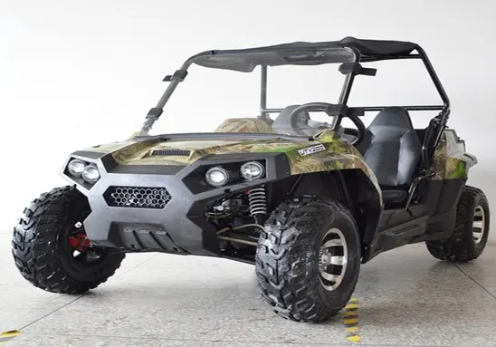
• An all-terrain vehicle(ATV), also known as a light utility vehicle (LUV), a quad bike, or simply a quad, as defined by the American National Standards Institute (ANSI); is a vehicle that travels on low-pressure tires, with a seat that is straddled by the operator, along with handlebars for steering control. As the name implies, it is designed to handle a wider variety of terrain than most other vehicles. Although it is a street-legal vehicle in some countries, it is not street-legal within most states, territories and provinces of Australia, the United States or Canada.
• By the current ANSI definition, ATVs are intended for use by a single operator, although some companies have developed ATVs intended for use by the operator and one passenger. These ATVs are referred to as tandem ATVs.
• The rider sits on and operates these vehicles like a motorcycle, but the extra wheels give more stability at slower speeds. Although most are equipped with three or four wheels, six-wheel models exists and existed historically for specialized applications. Multiple-user analogues with side-by-side seating are called utility terrain vehicles (UTVs) or side-by-sidesto distinguish the classes of vehicle.

Wheels and Tires

• ATVs have either three or four wheels. Tires are kept at a lower pressure than standard car or UTV tires.

Steering

• The operator can steer the ATV by using handlebars.

Seating and passenger capacity

• On an ATV, the operator is seated in a straddle position. ATVs are normally built for just one rider, some are made to carry the operator and one passenger.

Speed and handling

• ATVs are not “one-size-fits-all” and should be sized appropriately for the operator.When operated safely and correctly, ATVs offer a quick and nimble means of transportation over a variety of terrain.

Baja SAE:

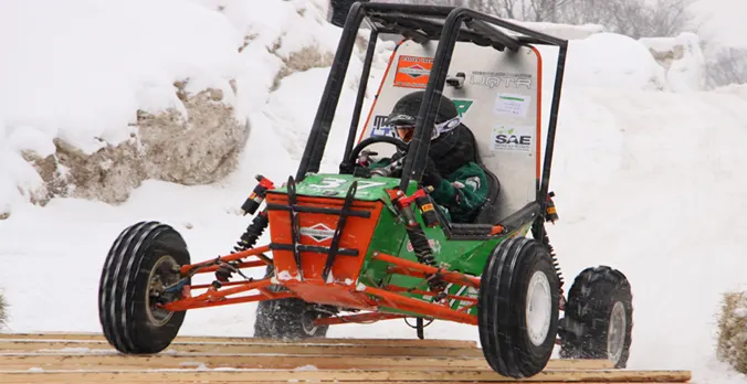
• Baja SAEis an Collegiate Design Series competition run by the Society of Automotive Engineers International (SAE International). Teams of students from universities all over the world design and build small off-road cars. The cars all have engines of the same specifications. As of 2018 the engine has been an unmodified Briggs & Stratton Model 19 Vanguard engine single-cylinder with a displacement of 305cc and power output of approximately 10 bhp (7.5 kW).

• All cars must adhere to SAE International's rules, and pass SAE's technical inspection and judging; a car may not race until all safety inspections are passed. Small engine manufacturer Briggs & Strattonsponsors Baja SAE teams by providing the SAE sanctioned engine free of charge, at a replacement rate of one engine for every two years in competition.
• There are multiple dynamic events, photographed by Official SAE Photographer Jethro Gaines of J. Gaines Studio, usually four per event, as well as a single four-hour endurance race. The dynamic events include hill climbs, sled pulls, maneuverability events, rock crawls, and suspension & traction events. Previously the cars had to be able to float and propel itself on water under its own power. This was changed from the 2012 competitions onward due to safety concerns.

Continuously Variable Transmission:

• Technically, a CVT is an automatic transmission because the driver isn't required to shift between the forward gears or operate a clutch pedal manually. But there are fundamental differences in both form and function between the two.
• Unlike a traditional automatic (or manual transmission, for that matter), a CVT does not have a fixed number of preset gears. Instead, it uses an unlimited number of gear ratios to accommodate the driving style and conditions at any given moment. Because it allows seamless changes without any hard shift points, a CVT transmission is often referred to as "single-speed" or "shiftless."
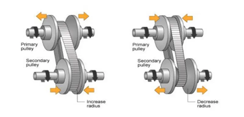
• A CVT achieves this infinite gear ratio flexibility by using two opposing cone-shaped pulleys with a chain or belt that runs between them. This setup is very similar to the way a chain operates across the gears of a bicycle.
• One cone is connected to the engine output shaft, while the other cone directs power to the driveshaft and drive wheels. Gear ratios change as the pulleys move closer and further apart, causing the chain or belt to move up and down the two cones' sides. This movement increases or decreases the diameter of the chain or belt, which alters the gear ratio based on the power needed. These real-time changes happen continually as the car is moving.

CVT Ratio:

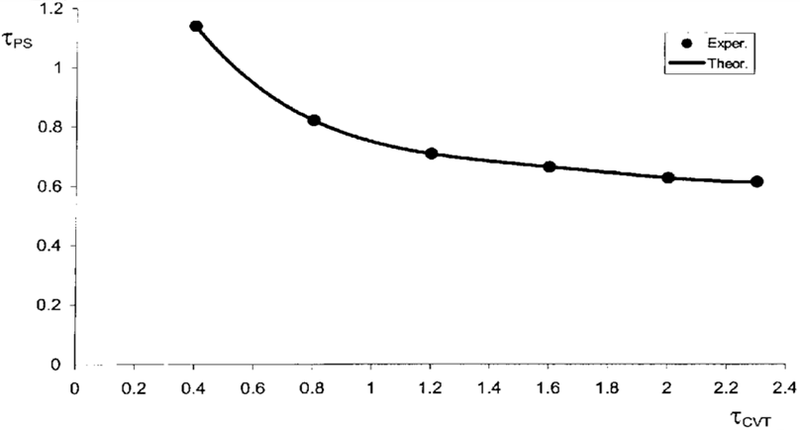
• In this work, theoretical and experimental results related to the power flow and efficiency of a power split continuously variable transmission (PS-CVT) system are reported. By means of two separate phases of operation, an original solution is studied that allows an increase in the transmission efficiency through the generation of a flow

cvtModel:

This is simscaps model. With the current vehicle parameters, the model is designed with gear reatio =10. For different vehicle parameters, you will need to tune the gear ratio.

Generic Engine:

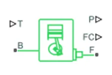
The Generic Engine block represents a general internal combustion engine. This block is a suitable generic engine for spark-ignition and diesel. Speed-power and speed-torque parameterizations are provided. A throttle physical signal input specifies the normalized engine torque. Optional dynamic parameters include crankshaft inertia and response time lag. A physical signal port outputs the engine fuel consumption rate based on the fuel consumption model that you choose. Optional speed and redline controllers prevent engine stall and enable cruise control.

Engine Speed, Throttle, Power, and Torque

• By default, the Generic Engine block uses a programmed relationship between torque and speed that is modulated by the throttle signal.
• The block evaluates engine power demand as a function of engine speed, g(Ω). The function provides the maximum power available for a given engine speed, Ω. The block parameters—Maximum power,Speed at maximum power,and Maximum speed— normalize this function to physical maximum torque and speed values.
• The normalized throttle input signal Tspecifies the actual engine power. The power is delivered as a fraction of the maximum power possible in a steady state at a fixed engine speed. It modulates the actual power delivered, P, from the engine: P(Ω,T) = Tg(Ω). The engine torque is τ = P/Ω.

Port:

Input

1. T— Normalized engine throttle level, unitless physical signal

Output

2. P— Instantaneous engine power, W physical signal (Power produced by the engine, in W.)
3. FC— Fuel consumption rate, kg/s physical signal (Fuel consumed by the engine, in kg/s.)

Conserving

1. B— Engine block
   mechanical rotational

• Mechanical rotational conserving port associated with the engine block. This is the base port. The engine block is the physical body that contains the piston cylinders.

2. F— Engine crankshaft
   mechanical rotational

• Mechanical rotational conserving port associated with the engine crankshaft. This is the follower port of engine. The crankshaft transmits the power generated from the combustion process. Typically, you attach a clutch and transmission at this port.

Simple Gear:

The Simple Gear block represents a gearbox that constrains the connected driveline axes of the base gear, B, and the follower gear, F, to corotate with a fixed ratio that you specify. You choose whether the follower axis rotates in the same or opposite direction as the base axis. If they rotate in the same direction, the angular velocity of the follower, ω_F, and the angular velocity of the base, ω_B, have the same sign. If they rotate in opposite directions, ω_F and ω_B have opposite signs. You can easily add and remove backlash, faults, and thermal effects.

Ideal Gear Constraint and Gear Ratio

• The kinematic constraint that the Simple Gearblock imposes on the two connected axes is

rFωF=rBωB

Port:

B — Base
rotational mechanical (Rotational mechanical conserving port associated with the base, or input, shaft.)

F — Follower
rotational mechanical (Rotational mechanical conserving port associated with the follower, or output, shaft.)

Engine Sensor:

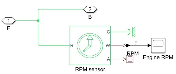
This model have subsystem block under cvtModel. Subsystem name is engine sensor.

Ideal Rotational Motion Sensor (RPM sensor):

• The Ideal Rotational Motion Sensor block represents an ideal mechanical rotational motion sensor, that is, a device that converts an across variable measured between two mechanical rotational nodes into a control signal proportional to angular velocity or angle. You can specify the initial angular position (offset) as a block parameter.
• The sensor is ideal since it does not account for inertia, friction, delays, energy consumption, and so on.
• Connections R and C are mechanical rotational conserving ports that connect the block to the nodes whose motion is being monitored. Connections W and A are physical signal output ports for velocity and angular displacement, respectively.
• The block positive direction is from port R to port C. This means that the velocity is measured as ω= ω_R – ω_C, where ω_R, ω_C are the absolute angular velocities at ports R and C, respectively.
• The Wrap angle to [0, 2*pi]parameter lets you control the angular displacement output range. When set to On, it keeps angular displacement within the range from 0 to 2π radians (360 degrees), regardless of the number of revolutions performed by the object and the direction of rotation. When set to Off, the output range is unrestricted.

Port:

Output:

W — Angular velocity, rad/s (physical signal). Physical signal output port for angular velocity.

A — Angular displacement, rad (physical signal). Physical signal output port for angular displacement.

Conserving

R — Rod (positive probe)
mechanical rotational

Mechanical rotational conserving port associated with the sensor positive probe.

C — Case (reference probe)
mechanical rotational

Mechanical rotational conserving port associated with the sensor negative (reference) probe.

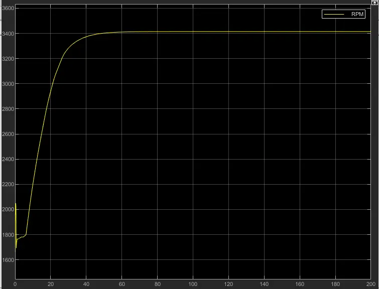
Fig 1: Engine RPM Graph.

CVT:

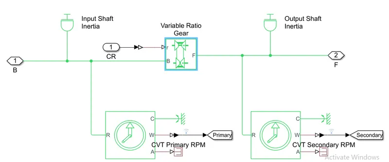
This model have subsystem block under cvtModel. Subsystem name is CVT(Continuously Variable Transmission).

Variable Ratio Gear:

• The Variable Ratio Transmission block represents a gearbox that dynamically transfers motion and torque between the two connected driveshaft axes, the base and the follower.
• When you choose to have the block ignore the dynamics of transmission compliance, it constrains the driveshafts to corotate with a variable gear ratio that you control. You can choose whether the follower axis rotates in the same or opposite direction as the base axis. If the follower and base axis rotate in the same direction, ω_Fand ω_B have the same sign. If the follower and base axis rotate in opposite directions, ω_F and ω_B have opposite signs.
• Transmission compliance introduces internal time delay between the axis motions. Unlike a gear, a variable ratio transmission does not act as a kinematic constraint. You can also control the torque loss caused by transmission and viscous losses.

Port:

Input-r — Input-to-output shaft velocity ratio, unitless
physical signal

Physical signal port associated with the input to output shaft ratio.

Conserving

B — Base driveshaft
mechanical rotational

Mechanical rotational conserving port associated with the base driveshaft.

F — Follower driveshaft
mechanical rotational

Inertia:

The Inertia block represents an ideal mechanical translational inertia that is described with the following equation:

T=Jdωdt

where:

• Tis inertia torque.
• Jis inertia.
• ωis angular velocity.
• tis time.

By default, the block has one mechanical translational conserving port. The block positive direction is from its port to the reference point. This means that the inertia torque is positive if inertia is accelerated in the positive direction.

In some applications, it is customary to display inertia in series with other elements in the block diagram layout. To support this use case, the Number of graphical ports parameter lets you display a second port on the opposite side of the block icon. The two-port variant is purely graphical: the two ports have the same angular velocity, so the block functions exactly the same whether it has one or two ports. The block icon changes depending on the value of the Number of graphical ports parameter.

Vehicle Body:

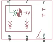
• The Vehicle Body block represents a two-axle vehicle body in longitudinal motion. The vehicle can have the same or a different number of wheels on each axle. For example, two wheels on the front axle and one wheel on the rear axle. The vehicle wheels are assumed identical in size. The vehicle can also have a center of gravity (CG) that is at or below the plane of travel.
• The block accounts for body mass, aerodynamic drag, road incline, and weight distribution between axles due to acceleration and road profile. Optionally include pitch and suspension dynamics. The vehicle does not move vertically relative to the ground.
• The block has an option to include an externally-defined mass and an externally-defined inertia. The mass, inertia, and center of gravity of the vehicle body can vary over the course of simulation in response to system changes.

Port:

Input

W — Headwind speed, m/s

beta — Road incline angle, rad

CG — Center of gravity, m
two-element vector

M — Mass, kg

J — External moment of inertia, kg*m^2

Output

V — Longitudinal velocity, m/s

NF — Front axle normal force, N

NR — Rear axle normal force, N

Conserving

H — Horizontal motion mechanical translational

Double Shoe Break:

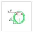
• The Double-Shoe Brake block represents a frictional brake with two pivoted rigid shoes that press against a rotating drum to produce a braking action. The rigid shoes sit inside or outside the rotating drum in a diametrically opposed configuration. A positive actuating force causes the rigid shoes to press against the rotating drum. Viscous and contact friction between the drum and the rigid shoe surfaces cause the rotating drum to decelerate.
• Double-shoe brakes provide high braking torque with small actuator deflections in applications that include motor vehicles and some heavy machinery. The model employs a simple parameterization with readily accessible brake geometry and friction parameters.
• You can also enable faulting. When faulting occurs, the belt will exert a user-specified force. Faults can occur at a specified time or due to an external trigger at port T.

Port:

Input

F — Actuating force.(physical signal)

T — External fault trigger.(physical signal)

Conserving

S — Drum shaft rotation. (rotational mechanical)

H — Heat flow. (thermal)

Tire:

• The Tire (Magic Formula) block models a tire with longitudinal behavior given by the Magic Formula , an empirical equation based on four fitting coefficients. The block can model tire dynamics under constant or variable pavement conditions.
• The longitudinal direction of the tire is the same as its direction of motion as it rolls on pavement. This block is a structural component based on the Tire-Road Interaction (Magic Formula)
• To increase the fidelity of the tire model, you can specify properties such as tire compliance, inertia, and rolling resistance. However, these properties increase the complexity of the tire model and can slow down simulation. Consider ignoring tire compliance and inertia if simulating the model in real time or if preparing the model for hardware-in-the-loop (HIL) simulation.

Port:

Input

N — Normal force(physical signal)

M — Magic formula coefficients (physical signal | vector | [B, C, D, E])

Output

S — Slip(physical signal)

Conserving

A — Axle(mechanical rotational)

H — Hub(mechanical translational)

Other Blocks Used:

1. Solver configuration – To specify the solver parameters before starting the simulation.
2. Signal builder – To input the brake, throttle and CVT Ratio.
3. Simulink to PS Converter – To convert Simulink signal to physical signal.
4. PS to Simulink Converter – TO convert physical signal to Simulink signal.
5. Mechanical Reference – To make sure all the components are clamped to the ground.
6. Rotational free end – the rotational free end block represents a mechanical rotational port that rotates freely, without torque.
7. Lookup Table – To insert the CVT values from the workspace
8. Step- To increase or decrease an input value for a defined time interval.

MAIN Model:

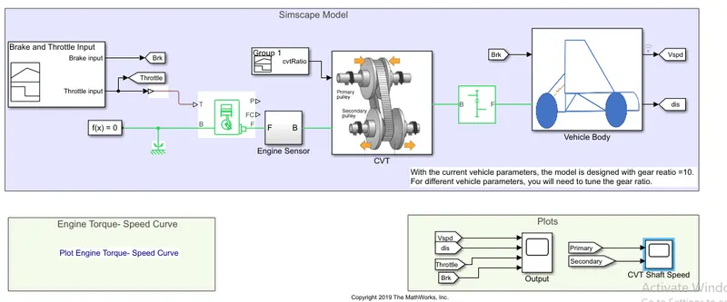
Fig 2: Baja ATV cvtModel

Steps:

1. The throttle signal is generated by signal builder block and connected with generic engine.
2. the engine will generate the output rpm which can be taken from crankshaft output.this speed will be given to the ideal rotational motion sensor the output rpm.
3. The same output speed will be given to a simple gear mechanism to redice the speed where the gear ratio is 10.
4. The cvt ratio is provided to the variable ratio transmission (cvt) block through signal builder.
5. The power from the cvt is inputted to the axle and the vehicle accelerates according to the speed.
6. Then the velocity is taken as output from the vehicle body for future analysis.

Input:

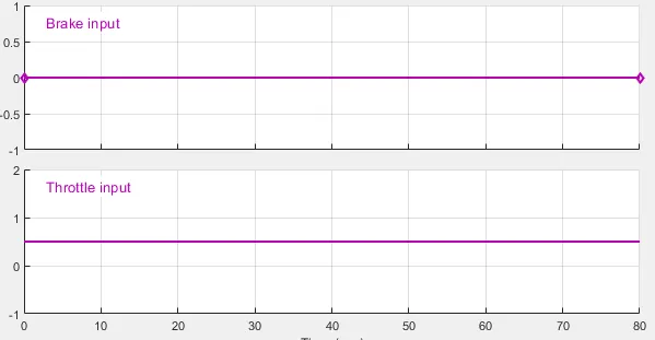
Fig 3: Break input and Throttle input signal.

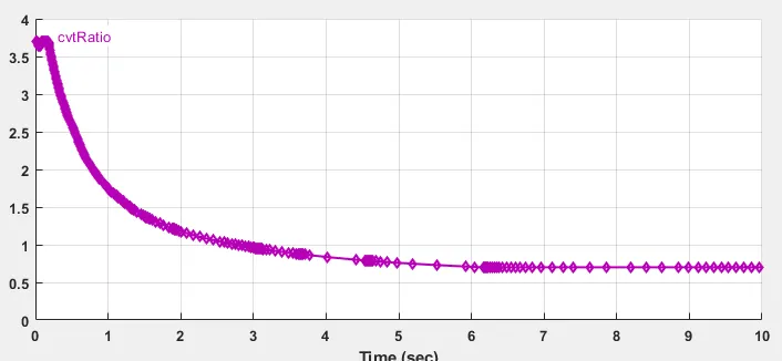
Fig 4: Baja ATV cvtRatio.

Output Result:

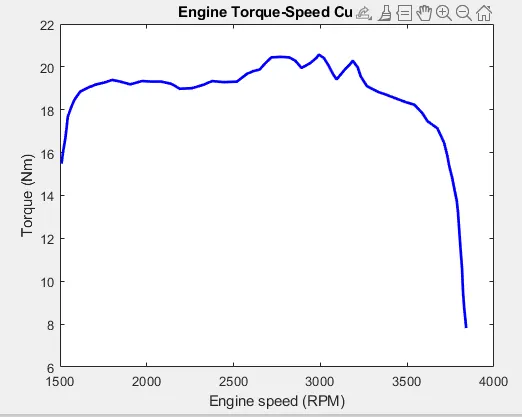
Fig 5: Engine Torque-speed Curve.

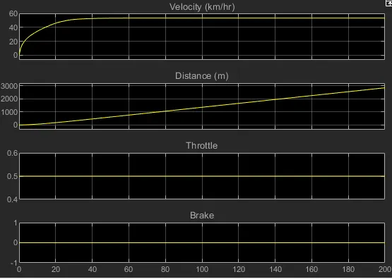
Fig 6: ATV cvtModel velocity, distance, throttle, break curve.

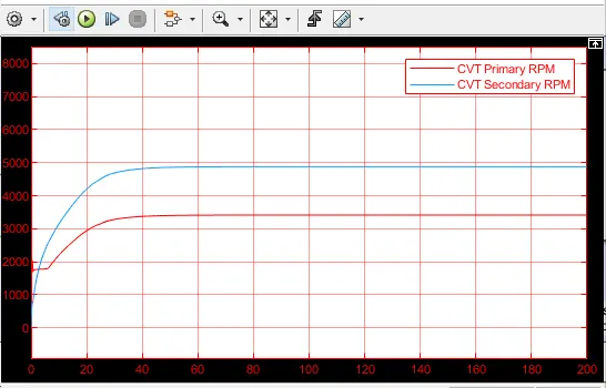
Fig 7: CVT Primary RPM vs CVT Secondary RPM.

cvtModel_Dashboard:

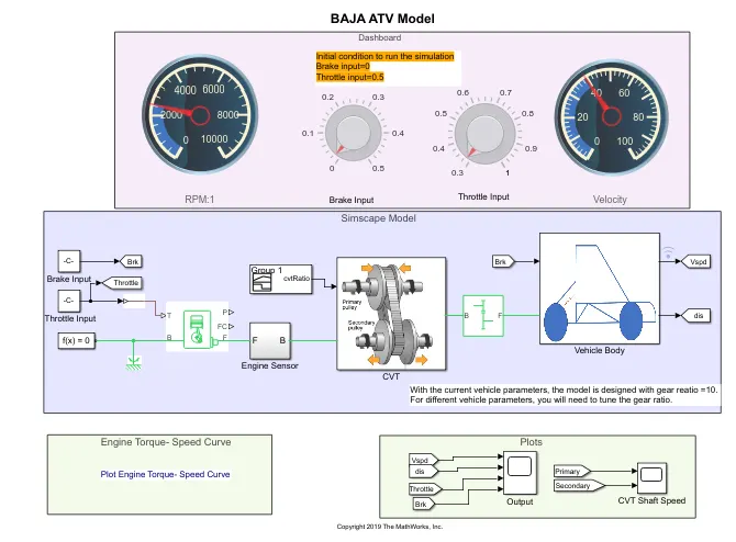
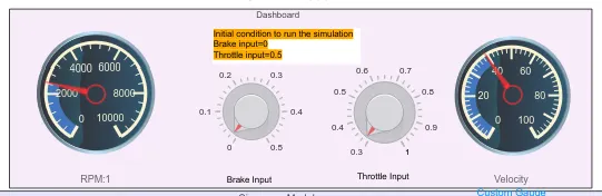
Fig 8: Baja ATV cvt Dashboard model.

Knob:

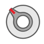
• First Knob connected with break input.
• Second Knob connected with throttle input.

The Knob block tunes the value of the connected block parameter to during simulation. For example, you can connect the Knob block to a Gain block in your model and adjust its value during simulation. You can modify the range of the Knob block's scale to fit your data. Use the Knob block with other Dashboard blocks to create an interactive dashboard to control your model.

Connect Dashboard Blocks

Dashboard blocks do not use ports to connect to model elements. To connect dashboard blocks to variables and block parameters, use connect mode. Connect mode facilitates the process of connecting dashboard blocks in your model, especially when you want to connect multiple blocks at once. To connect a single dashboard block, you can also use the Connection table in the block dialog box.

Circular Gauge:

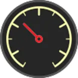
• First Circular Gauge connected with engine sensor subsystem block
• Second Circular Gauge connected with Vehicle body.

The Circular Gauge block displays the value of the connected signal on a circular gauge that you can design to look like a gauge in a real system.

The Circular Gauge block displays the instantaneous value of the connected signal throughout simulation. You can modify the range and tick values on the Circular Gauge block to fit your data. Use the Circular Gauge block with other dashboard blocks to build an interactive dashboard of controls and indicators for your model.

Connect Dashboard Blocks

Dashboard blocks do not use ports to connect to model elements. To connect dashboard blocks to signals in your model, use connect mode. Connect mode facilitates the process of connecting dashboard blocks in your model, especially when you want to connect multiple blocks at once. To connect a single dashboard block, you can also use the Connection table in the block dialog box.

Output Result:

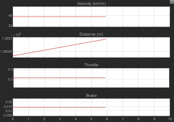
When throttle input increase then RPM and Velocity also increase simultaneously. cvtModel dashboard output curve . here break input ‘0’ and throttle input ‘o.3’.

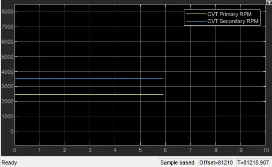
CVT Primary RPM and CVT Secondary RPM ratio output graph.

cvtModel_Dashboard_mapped:

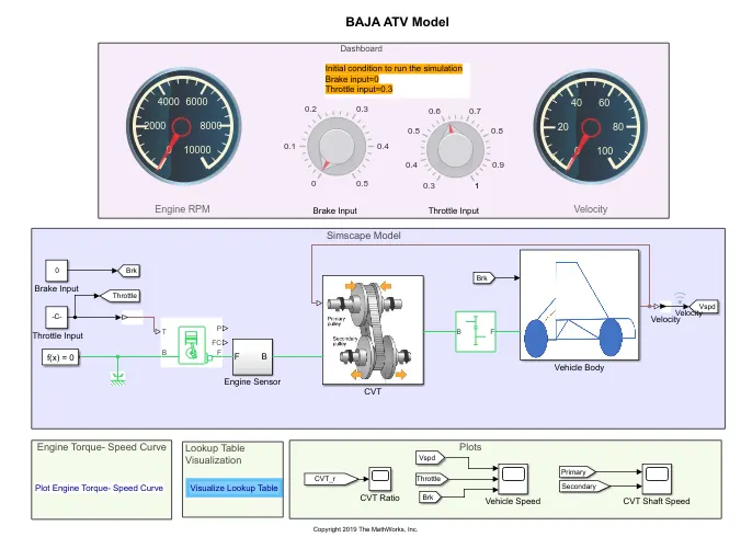
Fig 9: cvtModel_Dashboard_mapped.

Lookup Table:

Use blocks from the Lookup Tables library to model nonlinearity. Lookup table blocks use arrays of data to map input values to output values, approximating mathematical functions. To approximate a function in N variables, use the n-D Lookup Table block:

A lookup table is an array of data that maps input values to output values, thereby approximating a mathematical function. Given a set of input values, a lookup operation retrieves the corresponding output values from the table. If the lookup table does not explicitly define the input values, Simulink^® can estimate an output value using interpolation, extrapolation, or rounding, where:

• An interpolation is a process for estimating values that lie between known data points.
• An extrapolation is a process for estimating values that lie beyond the range of known data points.
• A rounding is a process for approximating a value by altering its digits according to a known rule.

A lookup table block uses an array of data to map input values to output values, approximating a mathematical function. Given input values, Simulink performs a “lookup” operation to retrieve the corresponding output values from the table. If the lookup table does not define the input values, the block estimates the output values based on nearby table values.

The following example illustrates a one-dimensional lookup table that approximates the function y = x³. The lookup table defines its output (y) data discretely over the input (x) range [-3, 3].

Lookup Table_Visualization.mat

%% Load and simulate the model

cvtModel_data

sim('cvtModel_data')

%% Visualize the lookup table

plot(vehicle_speed,cvtr,'r','LineWidth',2)

xlabel ('Vehicle Speed (km/hr)')

ylabel ('CVT Ratio')

title ('Lookup Table Visualization')

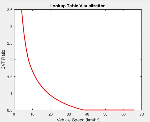
Fig 10: Lookup Table VisualizationVehicle speed graph.

CVT Ratio plot:

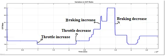
in this Baja ATV Model , the engine is pre set to run at 3300 rpm with the throttle value of 0.3 and the velocity at 45 KMPH. THE CVT RATIO for maximum speed of enginewas pre-defined as 2.3 and 1.8 respectively. when the simulaton is started in initial throttal value 0.3 is achived so that cvt ratio nearlyu 1.85.

Engine speed plot:

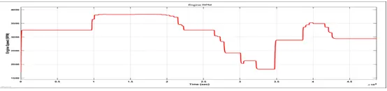
From the graph we can infer that the vehicle was first running at minimum RPM of 3300rpm and then throttal is applied (step-up) then breaking (step-down) then break is released so that engine rpm is inreased then breaking is applied.

CVT Speed reduction plot:

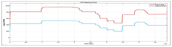
From the above graph we can understand that throttal is applied (step-up) anmd the kept constant the breaking is applied(step-down) then break is released so that engine speed is increased with increase in throttal input.

Speed vs Throttal plot:

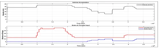
From the abovve plot we can infar that when throttal is applied the vehicle speed increasedand when break is applied vehicle speed decreased simultaneously.

Conclusion:

Here i was analysis how Baja ATV cvtModel is work. i understand engine throttal,speed velocity condition. i was understant how to work close loop. and understand An all-terrain vehicle(ATV), also known as a light utility vehicle (LUV), a quad bike, or simply a quad, as defined by the American National Standards Institute (ANSI); is a vehicle that travels on low-pressure tires, with a seat that is straddled by the operator, along with handlebars for steering control. As the name implies, it is designed to handle