Project
Aim
Carry out a system-level simulation of an all-terrain vehicle and to prepare a technical report explaining the model properties & comments on the results.
Introduction
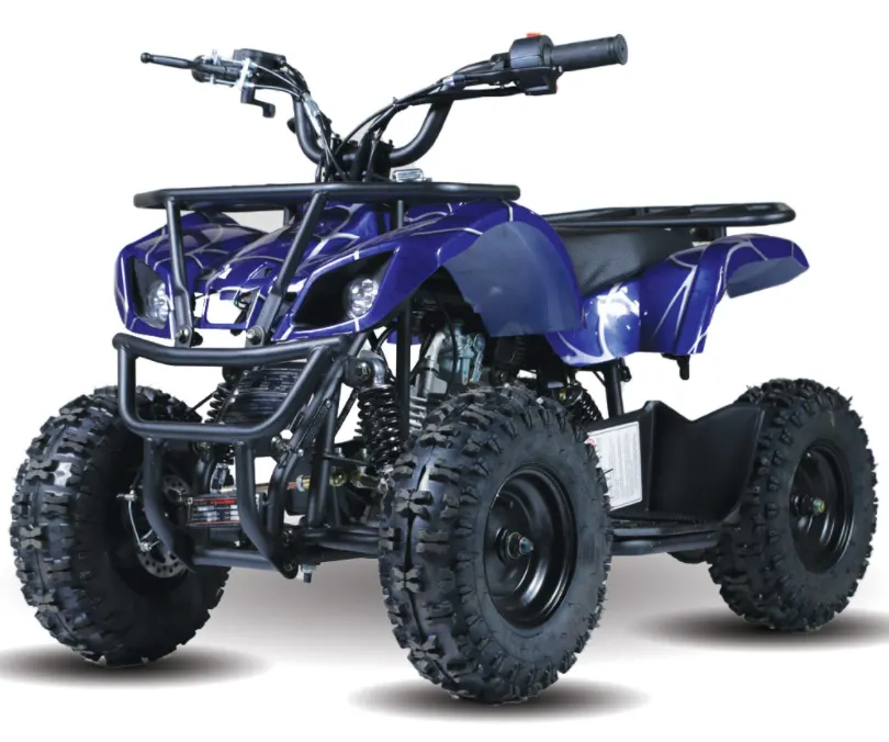
An all-terrain vehicle (ATV) is defined as a motorized off-highway vehicle designed to travel on four low-pressure or non-pneumatic tires and it consist of CVT transmission.
The CVT is an automatic transmission that uses two pulleys with a steel belt running between them. To continuously vary its gear ratios, the CVT simultaneously adjusts the diameter of the "drive pulley" that transmits torque from the engine and the "driven pulley" that transfers torque to the wheels.
Formula
Gear ratio =Tout/Tin or Nin/Nout
Tout=number of teeth on driven gear(gear connected to the axil)
Tin=number of teeth on driver gear(gear connected to the engine)
Nout=RPM on driven gear
Nin=RPM on driver gear
note
gear ratio decreases as the speed increases and vise versa
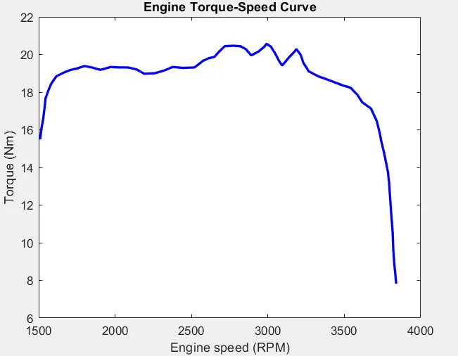
Torque is inversely proportional to speed. Thus, when speed increases, torque will decrease.
the above statement is evident from the graph below
Block used
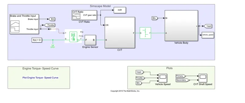
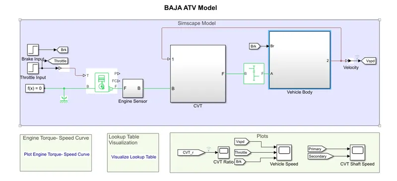
1)Generic Engine block
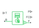
Represents a system-level model of spark-ignition and diesel engines suitable for use at initial stages of modeling when only the basic parameters are available. Optional idle speed and red line controllers are included.
The throttle input signal T lies between zero and one and specifies the torque demanded from the engine as a fraction of the maximum possible torque. If the engine speed falls below the Stall speed, the engine torque is blended to zero. If the engine speed exceeds the Maximum speed, the simulation stops and issues an error message.
Connections F and B are mechanical rotational conserving ports associated with the engine crankshaft and engine block, respectively. Connections P and FC are physical signal output ports through which engine power and fuel consumption rate are reported.
2)PS Lookup Table (1D)
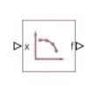
This block represents a physical signal converter whose input-output relationship is specified by a lookup table. The table grid must be in strictly ascending or strictly descending order, but the spacing can be nonuniform.
3)Variable Ratio Transmission
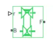
Represents a variable ratio gearbox such as implemented by mechanical belt CVT, electric, or hydraulic transmissions. The physical signal input r defines the ratio of input to output angular shaft velocities.
Connections B (base) and F (follower) are mechanical rotational conserving ports. Specify the relation between base and follower rotation directions with the Output shaft rotates parameter.
4)Simple Gear block

Represents a fixed-ratio gear or gear box. No inertia or compliance is modeled in this block. You can optionally include gear meshing, backlash, and viscous bearing losses.
Connections B (base) and F (follower) are mechanical rotational conserving ports. Specify the relation between base and follower rotation directions with the Output shaft rotates parameter. Optionally include thermal effects and expose thermal conserving port H by setting Friction model to a temperature-dependent setting.
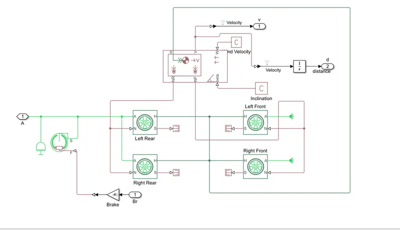
5)Vehicle Body
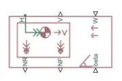
Represents a two-axle vehicle body in longitudinal motion. The block accounts for body mass, aerodynamic drag, road incline, and weight distribution between axles due to acceleration and road profile. The vehicle can have the same or a different number of wheels on each axle. Optionally include pitch and suspension dynamics or additional variable mass and inertia. The vehicle does not move vertically relative to the ground.
Connection H is the mechanical translational conserving port associated with the horizontal motion of the vehicle body. The resulting traction motion developed by tires should be connected to this port. Connections V, NF, and NR are physical signal output ports for vehicle velocity and front and rear normal wheel forces, respectively. Wheel forces are considered positive if acting downwards. Connections W and beta are physical signal input ports corresponding to headwind speed and road inclination angle, respectively. If variable mass is modeled, the physical signal input ports CG and M are exposed. CG accepts a two- element vector representing the x and y distance offsets from vehicle CG to additional load mass CG. M represents the additional mass. If both variable mass and pitch dynamics are included, the physical signal port J accepts the inertia of the additional mass about its own CG.
6)Tire

Represents the longitudinal behavior of a highway tire characterized by the tire Magic Formula. The block is built from Tire-Road Interaction (Magic Formula) and Simscape Foundation Library Wheel and Axle blocks. Optionally, the effects of tire inertia, stiffness, and damping can be included.
Connection A is the mechanical rotational conserving port for the wheel axle. Connection H is the mechanical translational conserving port for the wheel hub through which the thrust developed by the tire is applied to the vehicle. Connection N is a physical signal input port that applies the normal force acting on the tire. The force is considered positive if it acts downwards. Connection S is a physical signal output port that reports the tire slip. Optionally expose physical signal port M by setting Parameterize by to Physical signal Magic Formula coefficients. Physical signal port M accepts a four element vector corresponding to the B, C, D, and E Magic Formula coefficients.
7)Inertia

By default, the block has one mechanical translational conserving port. The block positive direction is from its port to the reference point. This means that the inertia torque is positive if inertia is accelerated in the positive direction.
In some applications, it is customary to display inertia in series with other elements in the block diagram layout. To support this use case, the Number of graphical ports parameter lets you display a second port on the opposite side of the block icon. The two-port variant is purely graphical: the two ports have the same angular velocity, so the block functions exactly the same whether it has one or two ports. The block icon changes depending on the value of the Number of graphical ports parameter.
8)Double-Shoe Brake
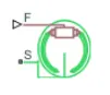
The Double-Shoe Brake block represents a frictional brake with two pivoted rigid shoes that press against a rotating drum to produce a braking action. The rigid shoes sit inside or outside the rotating drum in a diametrically opposed configuration. A positive actuating force causes the rigid shoes to press against the rotating drum. Viscous and contact friction between the drum and the rigid shoe surfaces cause the rotating drum to decelerate.
Double-shoe brakes provide high braking torque with small actuator deflections in applications that include motor vehicles and some heavy machinery. The model employs a simple parameterization with readily accessible brake geometry and friction parameters.
You can also enable faulting. When faulting occurs, the belt will exert a user-specified force. Faults can occur at a specified time or due to an external trigger at port T.
9)Step

The Step block provides a step between two definable levels at a specified time. If the simulation time is less than the Step time parameter value, the block's output is the Initial value parameter value. For simulation time greater than or equal to the Step time, the output is the Final value parameter value.
10)Signal builder
The Signal Builder block allows you to create interchangeable groups of piecewise linear signal sources and use them in a model. You can quickly switch the signal groups into and out of a model to facilitate testing. In the Signal Builder window, create signals and define the output waveforms.To open the window, double-click the block.
11)Gauge

The Circular Gauge block displays the value of the connected signal on a circular gauge that you can design to look like a gauge in a real system.
The Circular Gauge block displays the instantaneous value of the connected signal throughout simulation. You can modify the range and tick values on the Circular Gauge block to fit your data. Use the Circular Gauge block with other dashboard blocks to build an interactive dashboard of controls and indicators for your model.
12)Knob

The Knob block tunes the value of the connected block parameter to during simulation. For example, you can connect the Knob block to a Gain block in your model and adjust its value during simulation. You can modify the range of the Knob block's scale to fit your data. Use the Knob block with other Dashboard blocks to create an interactive dashboard to control your model.
Model 1
Common Inputs
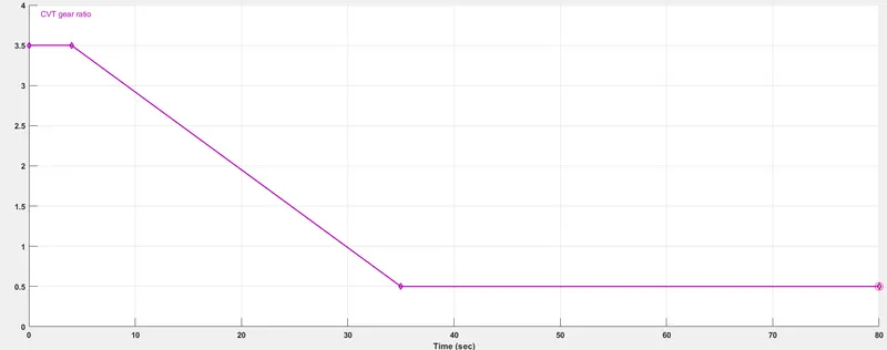
The CVT gear ratio is changing from 3.5 to 0.5
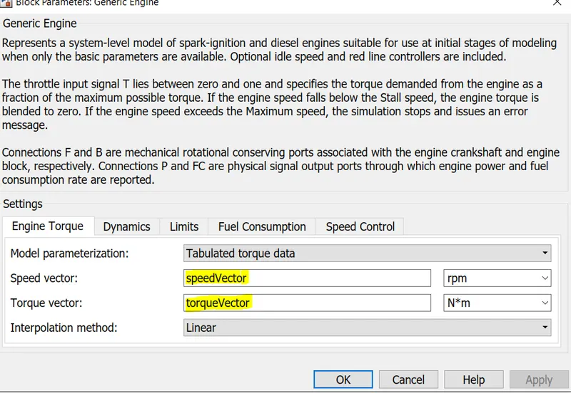
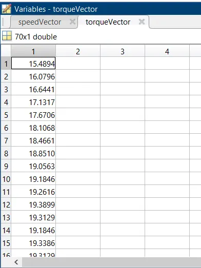
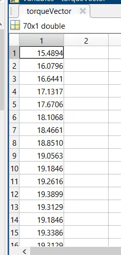
speedVector and torqueVector array are inputed into the generic engine block from the MATLAB which is preloaded
Results
Model 1 with signal builder
case1
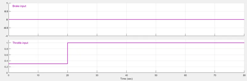
figure 1.1
The input data was given as shown in image above considering the brake input zero and the throttle increasing from 20th sec.
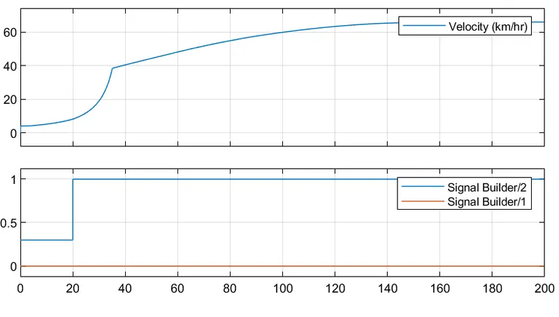
figure 1.2
here Signal Builder/2 is the throttle
Signal Builder/2 is the brake
from the above figure it is evident that when the throttle is increased suddenly at 20th sec the velocity(km/hr) also increased and thereafter it stabiles when the throttle is kept constant
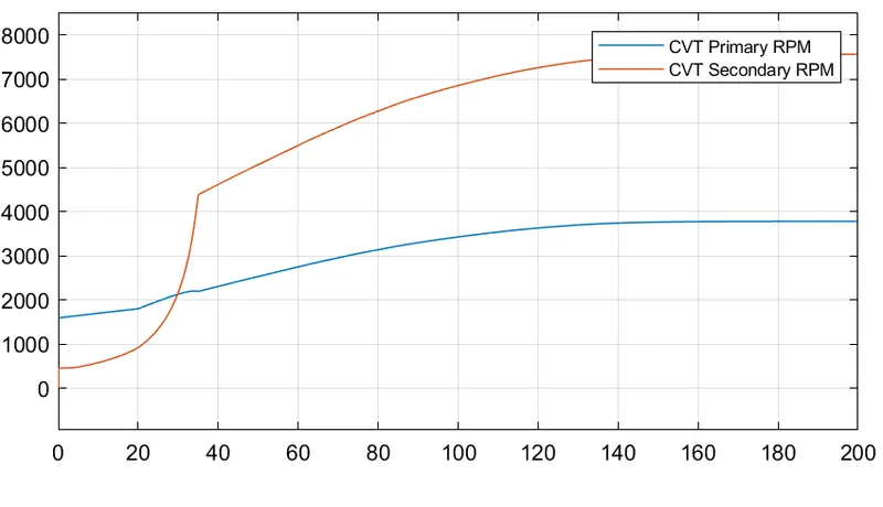
figure 1.3
By comparing the figure 1.2 and 1.3 it is visible that initially when the velocity(km/hr) was low ,primary pulley(driver) RPM (N1) was high as diameter(D1) is smaller compared to the secondary pulley (driven) RPM (N2)and diameter (D2) but thereafter once the velocity(km/hr) increased the secondary RPM (N2) increased as the diameter D2 decreased.
condition
When velocity is low
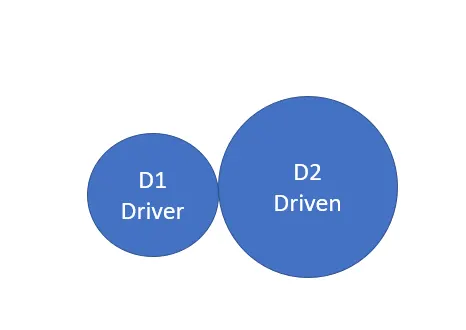
D1<D2
N1>N2
When velocity is greater
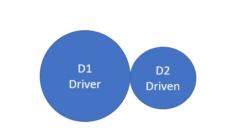
D1>D2
N1<N2
Model 1 with signal builder
Case2
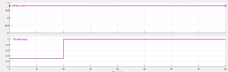
figure 2.1
The throttle input is kept same as the case1 but the only difference here is that the brakes have been applied
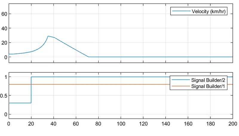
figure 2.2
When the brakes are applied it stopes the vechile and the velocity (km/hr) comes to zero
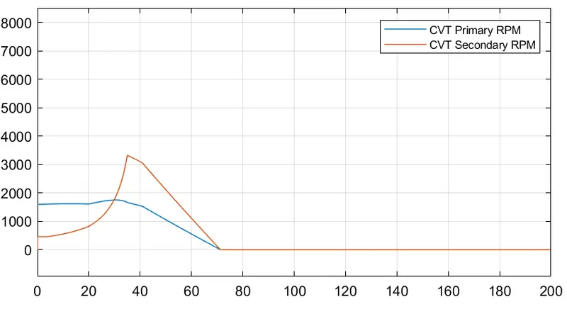
figure 2.3
By comparing the figure 2.2 and 2.3 it is visible that initially when the velocity(km/hr) was low ,primary pulley(driver) RPM (N1) was high as diameter(D1) is smaller compared to the secondary pulley (driven) RPM (N2)and diameter (D2) but thereafter once the velocity(km/hr) increased the secondary RPM (N2) increased as the diameter D2 decreased.
condition
When velocity is low
D1<D2
N1>N2
When velocity is greater
D1>D2
N1<N2
But as the brakes have been applied the CVT (continuously variable transmission) comes to rest which is evident from the plot
Model 1 with signal builder
case3
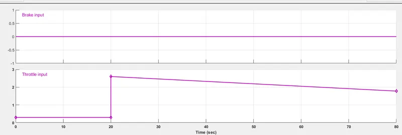
figure -3.1
The input data was given as shown in image above considering the brake input zero and the throttle increasing at 20th sec and therafter decreacing.
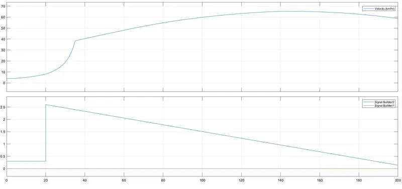
figure -3.2
from the above figure it is evident that when the throttle is increased suddenly at 20th sec the velocity(km/hr) also increased but thereafter when the throttle is decreased the velocity also decreases
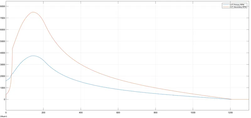
figure -3.3
By comparing the figure 3.2 and 3.3 it is visible that initially when the velocity(km/hr) was low ,primary pulley(driver) RPM (N1) was high as diameter(D1) is smaller compared to the secondary pulley (driven) RPM (N2)and diameter (D2) but thereafter once the velocity(km/hr) increased the secondary RPM (N2) increased as the diameter D2 decreased.
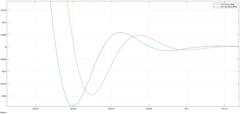
figure -3.4
figure 3.3 has been zoomed to show the evidence that the primary pully RPM N1 >secondary pully RPM N2 as the velocity (km/hr ) decreases. But the value should n
condition
When velocity is low
D1<D2
N1>N2
When velocity is greater
D1>D2
N1<N2
When velocity is low again as the throttle is decreased
D1<D2
N1>N2
Model2
Common Inputs
speedVector and torqueVector array are inputed into the generic engine block from the matlab which is preloaded
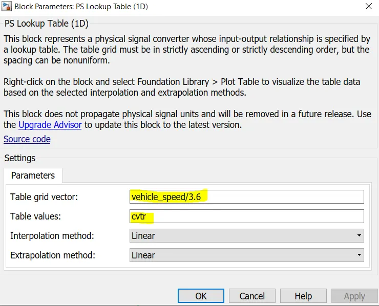
vechicle_speed/3.6 and cvtr values are entered via matlab which is preloaded to the look up table block.
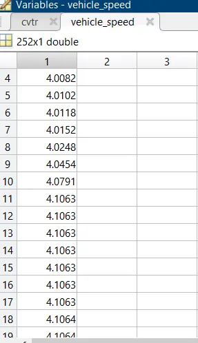
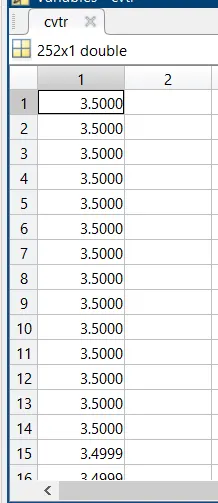
These values shown above is preloaded to MATLAB and is used to plot the graph as shown below using lookup table and is used as an input to the CVT ( continuously variable transmission ) block
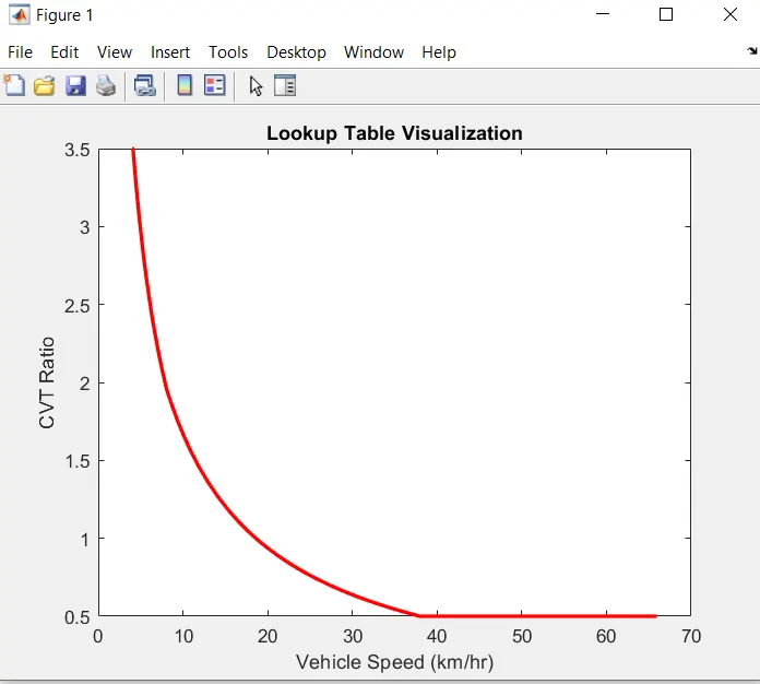
The CVT gear ratio is changing from 3.5 to 0.5
Results
Model 2 with lookup table
case 1
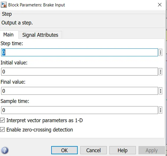
As brake has been not applied all above values remain 0
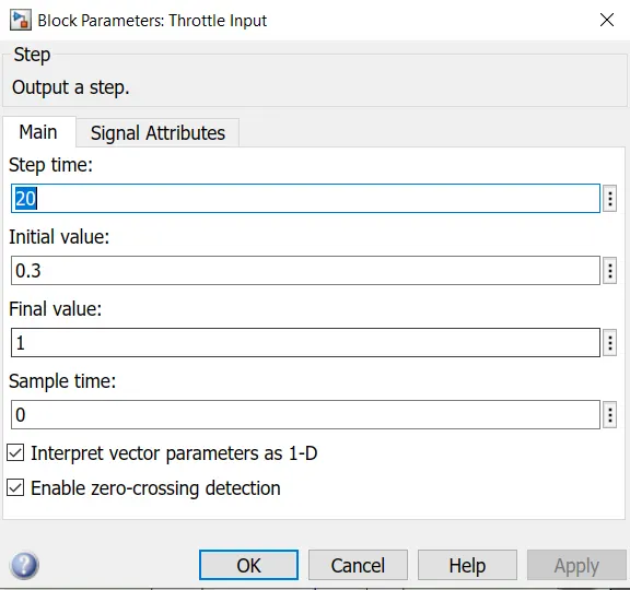
Throttle input step time is given as 20 which means that the throttle will start from 20sec
and the intial value is set as 0.3 and final value is set as 1
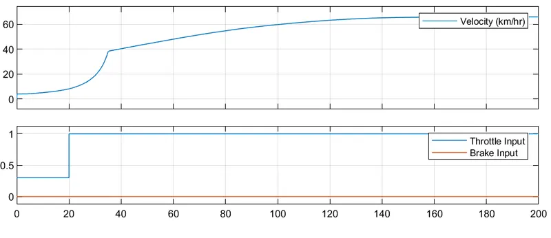
figure -4.1
from the above figure it is evident that when the throttle is increased suddenly at 20th sec the velocity(km/hr) also increased and thereafter it stabiles when the throttle is kept constant
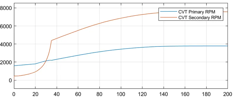
figure -4.2
By comparing the figure 4.1 and 4.2 it is visible that initially when the velocity(km/hr) was low ,primary pulley(driver) RPM (N1) was high as diameter(D1) is smaller compared to the secondary pulley (driven) RPM (N2)and diameter (D2) but thereafter once the velocity(km/hr) increased the secondary RPM (N2) increased as the diameter D2 decreased.
condition
When velocity is low
D1<D2
N1>N2
When velocity is greater
D1>D2
N1<N2
Model 2 with lookup table
case 2
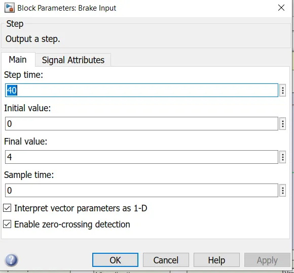
The brake step time was set to 40 upto the final value 4
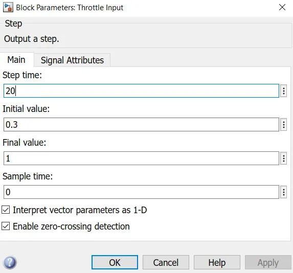
Throttle input step time is given as 20 which means that the throttle will start from 20sec
and the intial value is set as 0.3 and final value is set as 1
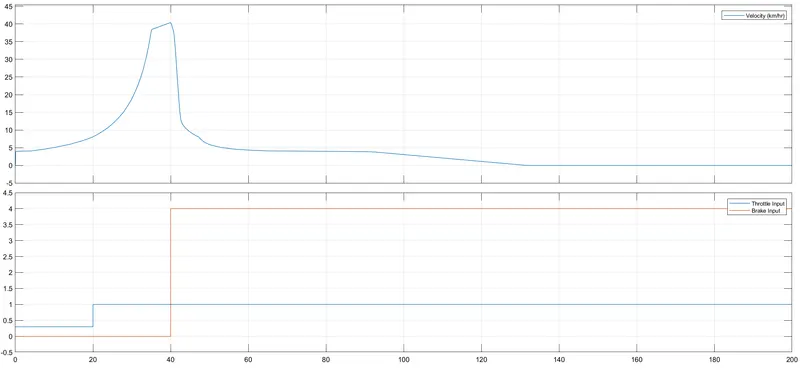
figure 5.1
from the above figure it is evident that when the throttle is increased suddenly at 20th sec the velocity(km/hr) also increased and at 40th sec the brake was applied hence we can see the velocity(km/hr) dropping
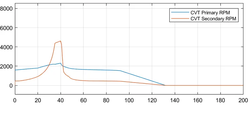
figure 5.2
By comparing the figure 5.1 and 5.2 it is visible that initially when the velocity(km/hr) was low ,primary pulley(driver) RPM (N1) was high as diameter(D1) is smaller compared to the secondary pulley (driven) RPM (N2)and diameter (D2) but thereafter once the velocity(km/hr) increased the secondary RPM (N2) increased as the diameter D2 decreased and after braking when the velocity(km/hr) was decreased ,primary pulley(driver) RPM (N1) was high as diameter(D1) is smaller compared to the secondary pulley (driven) RPM (N2)and diameter (D2).
condition
When velocity is low
D1<D2
N1>N2
When velocity is greater
D1>D2
N1<N2
When velocity is low again as the braking was done
D1<D2
N1>N2
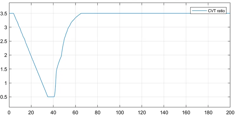
gear ratio decreases from 3.5 to 0.5 as the speed increases and after braking the speed decreases and the gear ration increases from 0.5 to 3.5 as the speed decreases.
example to prove the above statement
Gear ratio =Tout/Tin or Nin/Nout
Tout=number of teeth on driven gear(gear connected to the axil)
Tin=number of teeth on driver gear(gear connected to the engine)
Nout=RPM on driven gear
Nin=RPM on driver gear
low speed
Gear Ratio=Tout/Tin= 300/600=0.5
high speed
Gear Ratio=Tout/Tin= 100/600= 0.16 (output gear dia decreased hence higher RPM)
Model 3
common Inputs
speedVector and torqueVector array are inputed into the generic engine block from the matlab which is preloaded
vechicle_speed/3.6 and cvtr values are entered via matlab which is preloaded to the look up table block.
These values shown above is preloaded to MATLAB and is used to plot the graph as shown below using lookup table and is used as an input to the CVT ( continuously variable transmission ) block
The CVT gear ratio is changing from 3.5 to 0.5
Model 3 with dashboard and look up table
case 1
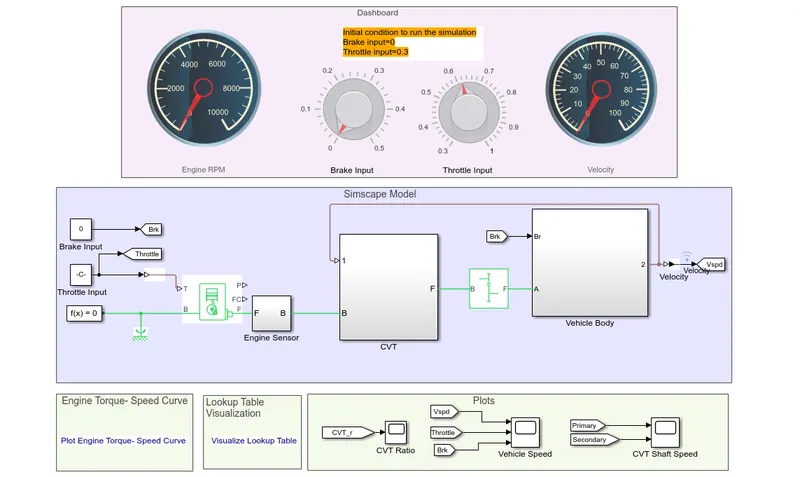
Result
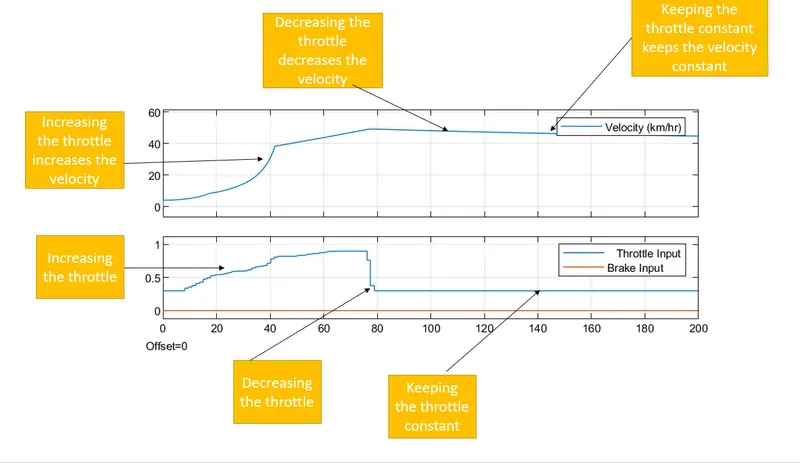
figure 6.1
The throttle knob was used to increase the throttle initially and later on the throttle was reduced using the same throttle know.
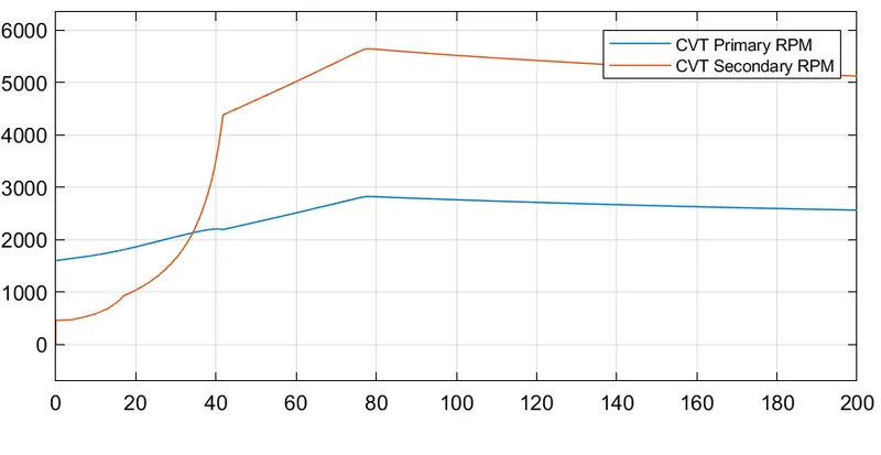
figure 6.2
from the figure 6.1 and 6.2 we can see that when throttleing was increased the primary pulley(driver) RPM (N1) was low as diameter(D1) is bigger compared to the secondary pulley (driven) RPM (N2)and diameter (D2) and vise versa once the throttleing was decreased
condition
When throttleing is increased
D1>D2
N1<N2
When throttleing is decreased
D1<D2
N1>N2
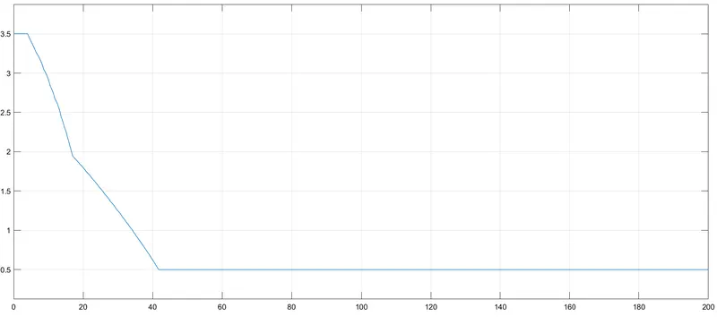
The gear ratio changes from 3.5 to 0.5
Model 3 with dashboard and look up table
case 2
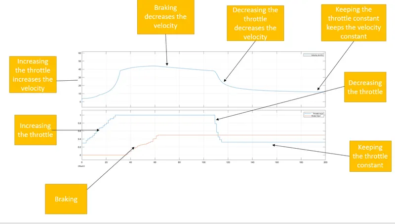
figure 7.1
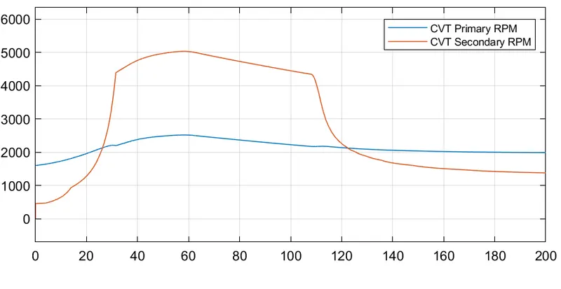
figure 7.2
from the figure 7.1 and 7.2 we can see that when throttleing was increased the primary pulley(driver) RPM (N1) was low as diameter(D1) is bigger compared to the secondary pulley (driven) RPM (N2)and diameter (D2) and vise versa while braking and once the throttleing was decreased.
condition
When throttleing is increased
D1>D2
N1<N2
while braking and decreacing the throttleing
D1<D2
N1>N2
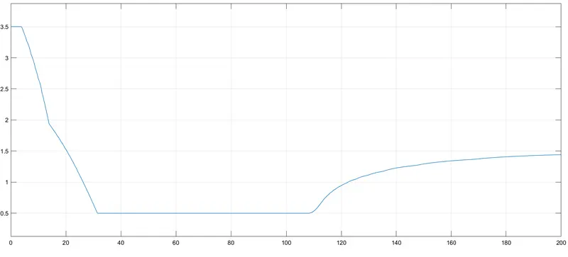
gear ratio decreases from 3.5 to 0.5 as the speed increases and after braking the speed decreases and the gear ration increases from 0.5 to 3.5 as the speed decreases.
example to prove the above statement
Gear ratio =Tout/Tin or Nin/Nout
Tout=number of teeth on driven gear(gear connected to the axil)
Tin=number of teeth on driver gear(gear connected to the engine)
Nout=RPM on driven gear
Nin=RPM on driver gear
low speed
Gear Ratio=Tout/Tin= 300/600=0.5
high speed
Gear Ratio=Tout/Tin= 100/600= 0.16 (output gear dia decreased hence higher RPM)
Model 4
The model 3 is same as the model 1 the only difference is that throttle input and brake input are controlled by the knob.
Model 4 with dashboard and signal builder.
common inputs
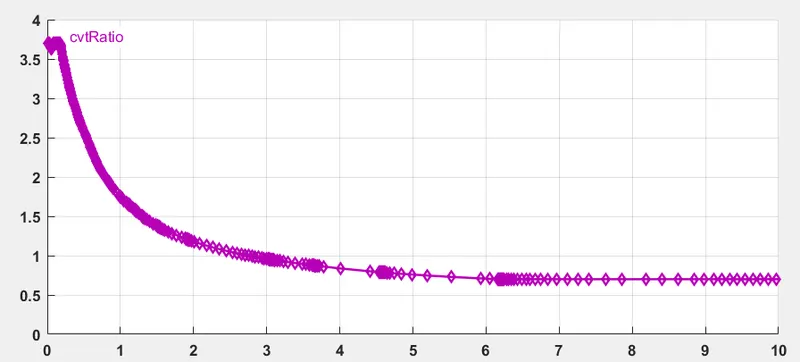
The CVT gear ratio is changing from 3.5 to 0.5
speedVector and torqueVector array are inputed into the generic engine block from the MATLAB which is preloaded
case1
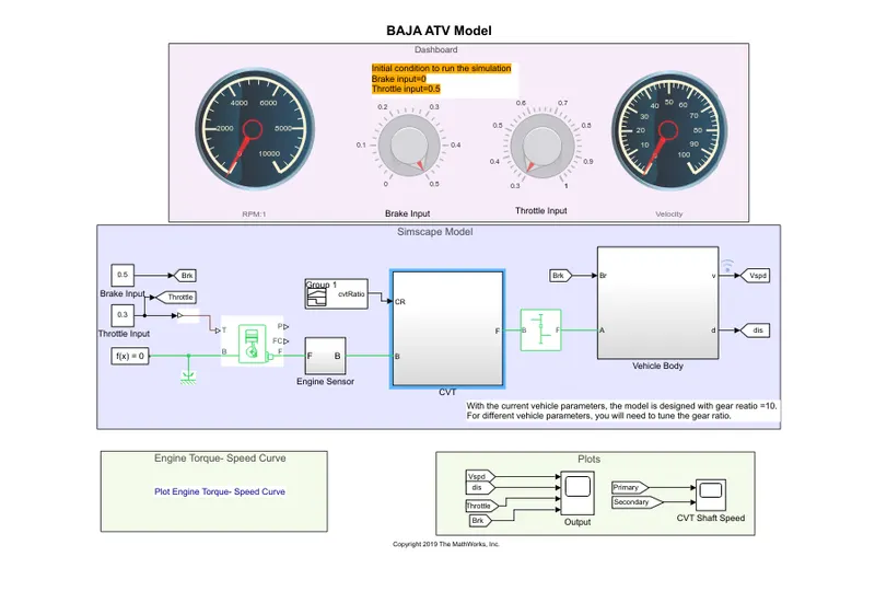
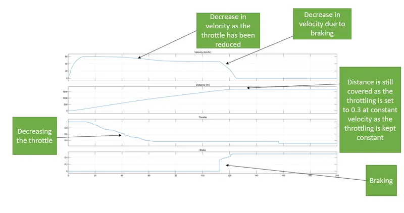
figure 8.1
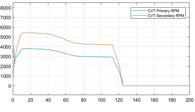
figure 8.2
By comparing the figure 8.1 and 8.2 it is visible that initially when the velocity(km/hr) was low ,primary pulley(driver) RPM (N1) was high as diameter(D1) is smaller compared to the secondary pulley (driven) RPM (N2)and diameter (D2) but thereafter once the velocity(km/hr) increased the secondary RPM (N2) increased as the diameter D2 decreased and after braking the
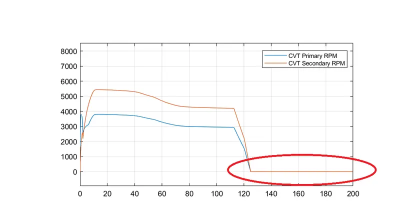
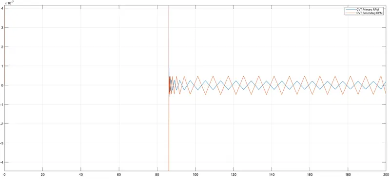
Throttling is kept constant at 0.3 and by zooming into the the figure 8.2 we can see that D1 alomost equal to D2 and the N1 is almost equal to N2 of the two pulley of the CVT hence we have achived a plot as shown above.
screen shots of the Sub- systems in expanded view
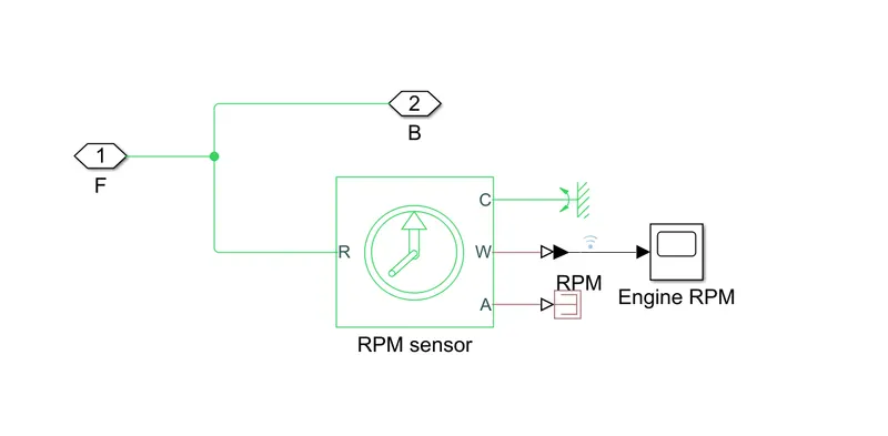
Engine sensor
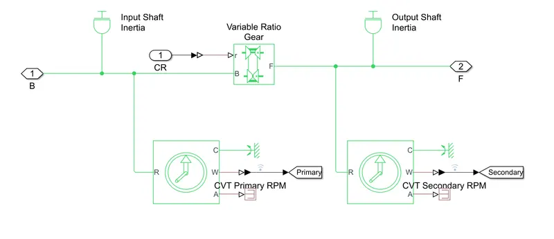
CVT system
Vechile body