Project
BAJA ATV (ALL TERRAIN VEHICLE) ANALYSIS USING SIMULINK:
AIM:
To study the analysis the BAJA ALL (All Terrain Vehicle) model usinh simulink.
OBJECTIVE:
- To prepear a techinical report of BAJA ATV model with and without lookup table.
THEORY:
ALL TERRAIN VEHICLE:
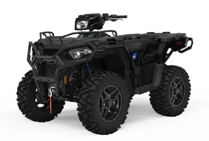
An all-terrain vehicle (ATV), also known as a quad (cycle), three-wheeler, four-track, four-wheeler, or quadricycle, as defined by the American National Standards Institute (ANSI) is a vehicle that travels on low-pressure tires, with a seat that is straddled by the operator. along with handlebars for steering control. It is designed to handle a wider variety of terrain than most other vehicles.
BAJA ATV (SAE):
I The BAJA SAE Series is an event for the undergraduate engineering students, organized globally by the Society of Automotive Engineers, USA. The event originated in the name of Mini - BAJA, in the year 1976 at University of Carolina. Since then, the event has spanned across six countries-USA, Mexico, South Africa, Korea, Brazil and India. The BAJA SAE tasks the students to design, fabricate and validate a single seater four-wheeled off road vehicle to take part in series of events spread over a course of 3 days that test the vehicle for the sound engineering practices that have gone into it, the agility of the vehicle in terms of gradeability, speed, acceleration and manoeuvrability characteristics and finally its ability to endure that back breaking durability test.
MAJOR COMPONENTS USED IN THIS SIMULATION :
GENERIC ENGINE:
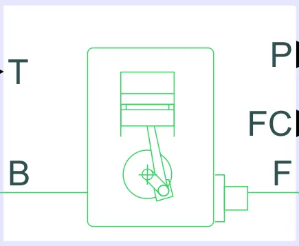
The Generic Engine block represents a general Internal Combustion (IC) Engine which is a type of Spark Ignition (SI-Petrol) or Compression Ignition (CI-Diesel). The speed torque and speed power parameters are provided.
PORTS,
i. B-Rotational Conserving Port representing the Engine Block
ii. F-Rotational Conserving Port representing the Engine Crankshaft
iii. T- Physical signal input port specifying the normalized engine throttle level
iv. P- Physical signal output port reporting the instantaneous engine power, in W v. FC - Physical signal output port reporting the fuel consumption rate, in kg/s
SIMPLE GEAR :
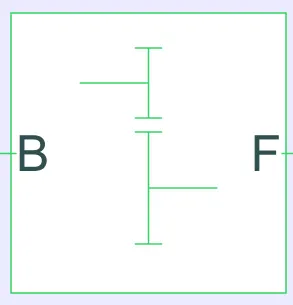
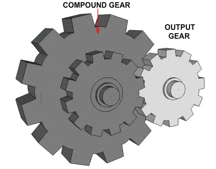
The simple gear is combination of a driver and driven gear where the speed is reduced by the gear ratio. The gear ratio is
defined as.
Gear Ratio = Follower. Gear. Speed / Base. Gear. Speed
PORTS,
i. B-Base Gear or Driver Gear
ii. F- Follower Gear or Driven Gear
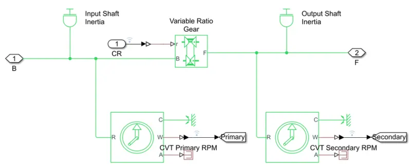
CVT TRANSMISSION :
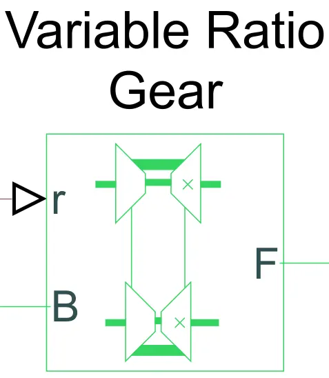
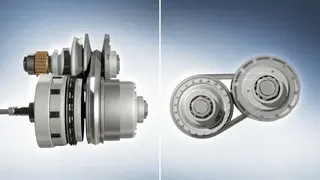
In CVT (Continuous Variable Transmission) the variable diameter pulley plays a vital role in transmission. Variable diameter pulleys must always come in pairs. One of the pulleys, known as the drive pulley (or driving pulley), is connected to the crankshaft of the engine. The driving pulley is also called the input pulley because it's where the energy from the engine enters the transmission. The second pulley is called the driven pulley because the first pulley is turning it. As an output pulley, the driven pulley transfers energy to the driveshaft.
The distance between the centre of the pulleys to where the belt makes contact in the groove is known as the pitch radius. When the pulleys are far apart, the belt rides lower and the pitch radius decreases. When the pulleys are close together, the belt rides higher and the pitch radius increases. The ratio of the pitch radius on the driving pulley to the pitch radius on the driven pulley determines the gear. when the pitch radius is small on the driving pulley and large on the driven pulley, then the rotational speed of the driven pulley decreases, resulting in a lower "gear." When the pitch radius is large on the driving pulley and small on the driven pulley, then the rotational speed of the driven pulley increases, resulting in a higher "gear." Thus, in theory, a CVT has an infinite number of "gears" that it can run through at any time, at any engine or vehicle speed.
PORTS,
i. B-Base Pulley or Drive Pulley
ii. F- Follower Pulley or Driven Pulley iii. r-Variable Transmission Ratio (Input)
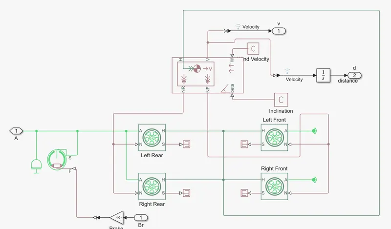
VEHICLE BODY :
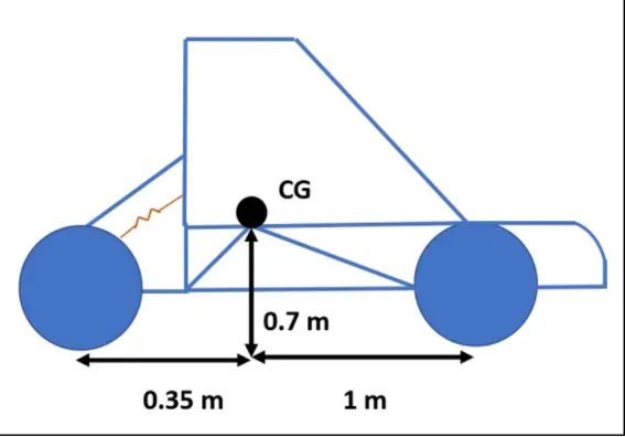
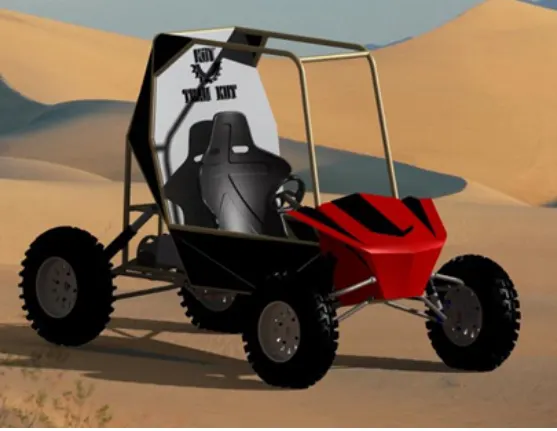
Two-axle vehicle with longitudinal dynamics and motion and adjustable mass, geometry, and drag properties. The vehicle can have the same or a different number of wheels on each axle. For example, two wheels on the front axle and one wheel on the rear axle. The vehicle wheels are assumed identical in size. The vehicle can also have a centre of gravity (CG) that is at or below the plane of travel.
PORTS,
i. NR - Rear Axle Normal Force (N)
ii. NF-Front Axle Normal Force (N)
iii. Beta-Road Incline Angle (rad)
iv. V-Longitudinal Velocity (m/s)
v. W - Head Wind Speed (m/s) vi. H- Horizontal Motion
DOUBLE SHOE BRAKE:
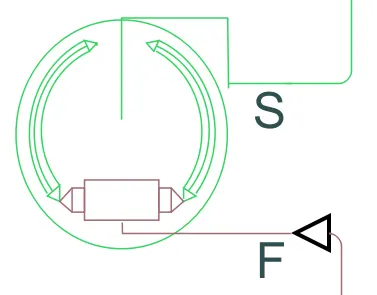
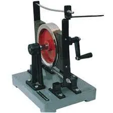
The Double-Shoe Brake block represents a frictional brake with two pivoted rigid shoes that press against a rotating drum to produce a braking action. The rigid shoes sit inside or outside the rotating drum in a diametrically opposed configuration. A positive actuating force causes the rigid shoes to press against the rotating drum. Viscous and contact friction between the drum and the rigid shoe surfaces cause the rotating drum to decelerate.
PORTS,
i.S-Rotational conserving port associated with the rotating drum shaft.
TIRE :
ii. F- Physical signal input port associated with the applied actuating force
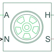
The vehicle body is connected to 4 tires each per axle to move the vehicle according to the power input to the axle.
PORTS.
i. N-Normal Force
ii. S-Tire Slip
iii. A-Axle
iv. H-Mechanical translational port associated with the wheel hub that transmits the thrust generated by the tire to the remainder of thevehicle.
TYPES OF MODEL:
i. BAJA ATV model without Dashboard
ii. BAJA ATV model with Dashboard
iii. BAJA ATV model-Lookup Table Data Extraction
iv. BAJA ATV model-Mapped Lookup Table without Dashboard
v. BAJA ATV model-Mapped Lookup Table with Dashboard
i. BAJA ATV model without Dashboard
MAIN MODEL:
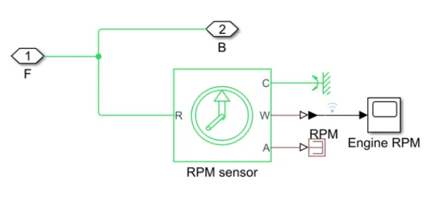
ENGIN SENSOR:
CVT SYSTEM:
VECHILE BODY:
FLIOW PROCESS:
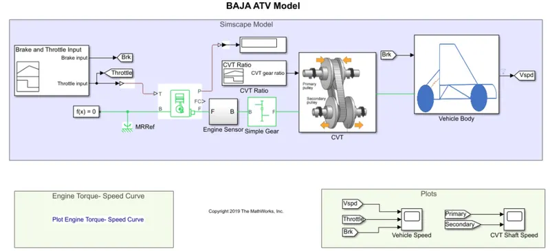
1. The throttle signal is genrated by signal builder block and inputted to generic engine.

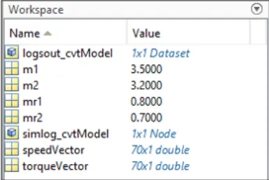
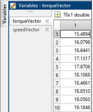
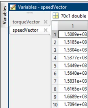
2.The Torque and speed vector are inputted from the MATLAB workspace
iii.The engine will generate the output rpm which can be taken from the crankshaft output. This speed will be given to the Ideal Rotational Motion Sensor to sense the output rpm.
iv.The same output speed will be given to a simple gear mechanism to reduce the speed where the Gear Ratio is '4".
v.Then the output speed from the gear reducer will be given to the Variable Ratio Transmission block (CVT).
vi.The CVT ratio is provided to the Variable Ratio Transmission (CVT) block through Signal Builder
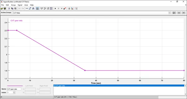
vii. The speed is controlled by the variable CVT ratios and the controlled output speed is inputted to the vehicle axle.
viii. The brake signal is generated by the signal builder and inputted to the vehicle body (Double Shoe Brake) for applying the brake to axle.

ix.The power from the CVT is inputted to the axle and the vehicle accelerates according to the speed.
x.Then the Velocity is taken as output from the vehicle body for further analysis.
RESULTS:
TORQUE SPEED PLOT :
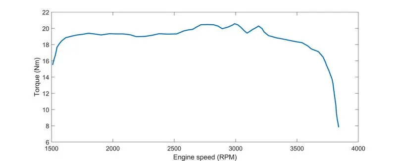
The torque and speed are inputted from the MATLAB workspace window to the generic engine block to generate the output RPM accordingly. This plot is common for all the cases because it's a default input to the engine.
ENGINE SPEED PLOT:
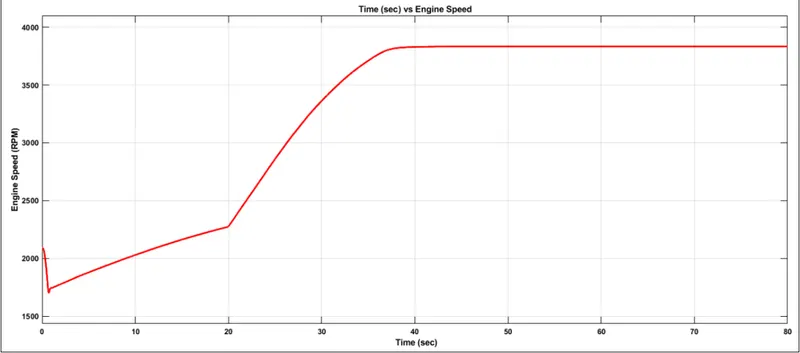
Here we can see the engine rpm genrated acordingly w.r.t to the throttle spped and torque input.
ENGINE SPEED VS GEAR REDUCTION SPEED PLOT:
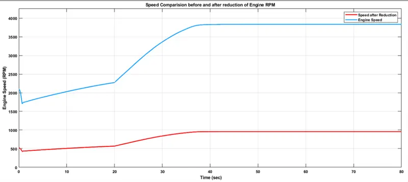
Here we can see that the engine speed is reduced by the Gear Ratio '4: For verification I calculated the maximum RPM, Maximum RPM (Before Reducing) = 3833 rpm
CVT SPEED REDUCTION PLOT:
The engine reduced speed is controlled by various CVT Ratios. For verification I had calculated the maximum RPM,
Maximum RPM (Before Reducing) = 958.25 rpm
The reduced maximum rpm is 958.25 rpm which can be verified from the plot.
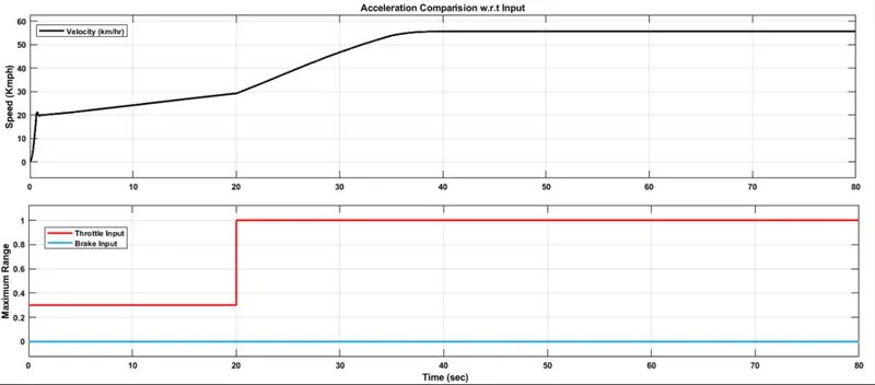
SPEED vs THROTTLE PLOT,
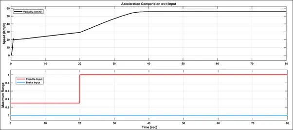
From the graph we can infer that the brake is not applied during the drive cycle and the Throttle is constant (0.3) till 20 sec and being increased from 0.3 to 1 from 20 sec where it remains constant throughout. With increase in throttle the vehicle speed also increases.
ACCELERATION PLOT
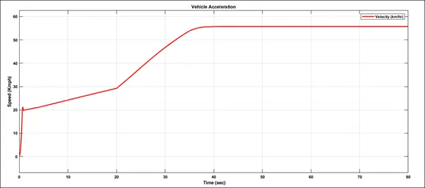
From the above plot we can infer that the vehicle is accelerated from 0-20 Kmph and then gradually increases then it’s accelerated to 55.74 Kmph where it remains constant throughout the cycle.
ii. BAJA ATV model with Dashboard.
MAIN MODEL
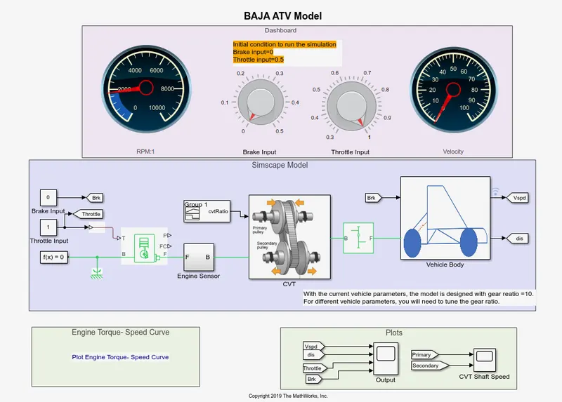
DASHBOARD MODEL:
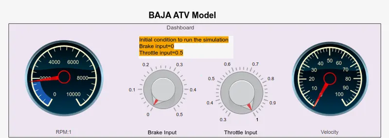
FLOW PROCESS:
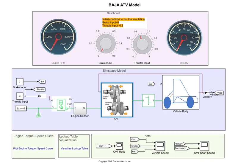
The model workflow process is same as the process of ‘BAJA ATV model without Dashboard’ but the Throttle and Brake inputs are controlled by the user with the Knob.
RESILTS:
ENGINE SPEED PLOTS,
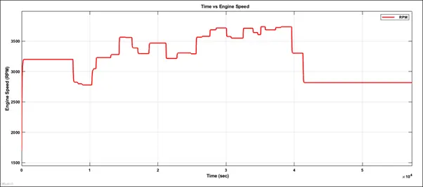
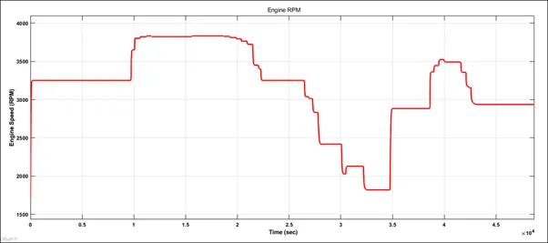
Here the engine speed is generated according to the inputs like throttle, break, torque and speed vectors. The runtime is not defined so that the Throttle and Break are controlled by the user. The step up is throttle and step down are break inputs.
ENGINE SPEED vs GEAR REDUCTION SPEED PLOT,
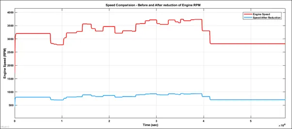
Here we can see that the engine speed is reduced by the Gear Ratio ‘4’. For verification I calculated the constant RPM (42000-50000 sec),
Maximum RPM (Before Reducing) = 2759.3 rpm
CVT SPEED REDUCTION PLOT,
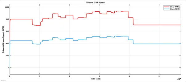
The engine reduced speed is controlled by various CVT Ratios. For verification I had calculated the constant RPM (42000-50000 sec),
Maximum RPM (Before Reducing) = 689.825 rpm
SPEED vs THROTTLE PLOT,
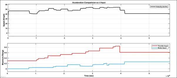
From the graph we can infer that the vehicle is accelerating while throttle is applied (Step Up) and decelerated while break is applied (Step Down).
ACCELERATION PLOT,
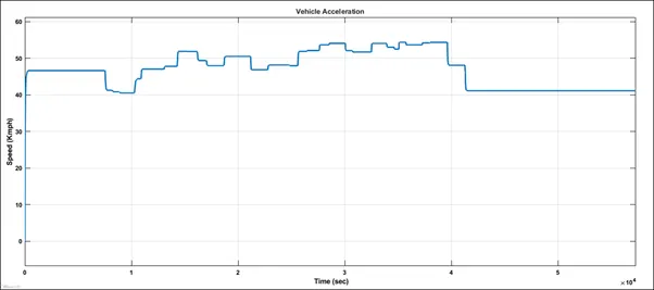
From the graph we can infer that the vehicle is accelerated to 46 Kmph initially and then the state changes when the user controls the throttle and brake knobs. The step-up and step-down are acceleration and deceleration respectively. The linear one is the constant speed so no changes in throttle or braking.
iii. BAJA ATV model-Lookup Table Data Extraction
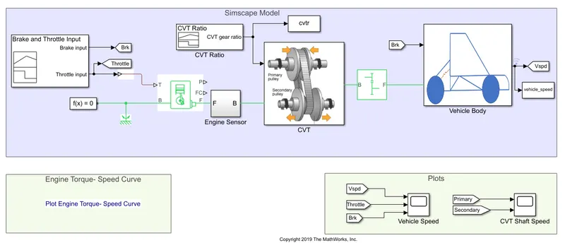
FLOW PROCESS :-
The model workflow process is same as the process of ‘BAJA ATV model without Dashboard’. The small addition is here the CVT Ratio and Vehicle Speed data are extracted using ‘To Workspace’ block.
RESULTS :-
The results are same as ‘BAJA ATV model without Dashboard’ but an additional output is the CVT Ratio and Vehicle Velocity to the Workspace.
iv. BAJA ATV model-Mapped Lookup Table without Dashboard
CVT BLOCK:
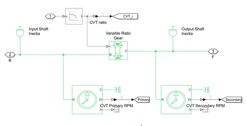
PROCESS:
- The Model workflow is same as the process of BAJA ATV model without Dashboard.
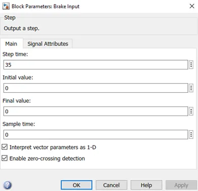
- Instead of Signal Builder blocks for Brake and throttle input the step blocks are used. At 35 sec the brake input will take a step of value 0.
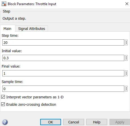
- The Throttle input is 20 sec throttle input will increases from 0.3-1 then remains constant throughout.
- And instead of Signal Builder Block for CVT Ratio the 2-D Lookup table is used. The interpolation and extrapolation methods are set to linear.
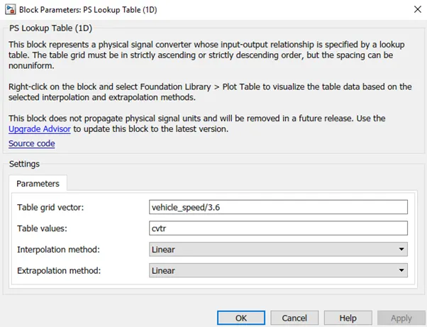
- At last the vehicle speed output is given as feedback tothe 2-D lookup table so that we can verify that the velocity of the vehicle is changing perfectly when the CVT Ratio changes. The vehicles speed is converted to m/s from kmph.
RESULTS:
CVT Ratio vs Vehicle Speed:
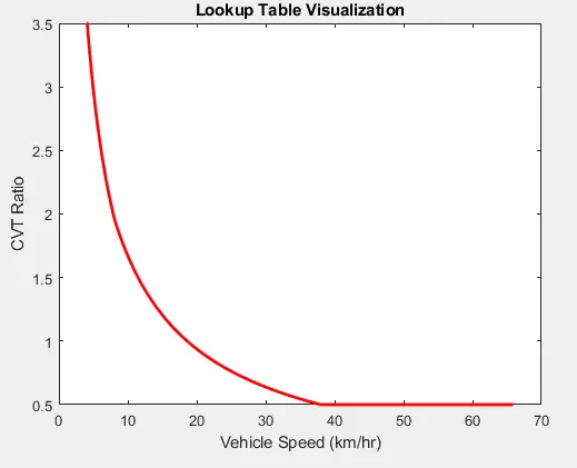
In the above plot is a value of the lookup table visualization
CVT RATIO PLOT,
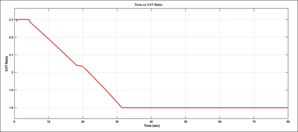
- 0 to 5 km/hr, the CVT ratio is constant at 3.5.
- 5 to 35 km/hr, the CVT ratio is drops down to 0.5.
- 35 km/hr onwards, the CVT ratio is constant at 0.5.
Hence, we can conclude that the vehicles accelerates, decelerates and remains constant when the CVT Ratio is being varied.
CVT RATIO vs VEHICLE VELOCITY,
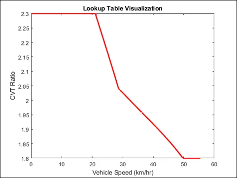
Here the CVT Ratio changes from 2.3 – 1.8 and the velocity value also changes w.r.t to the CVT Ratio. Hence, we can conclude that the vehicle accelerates, decelerates and remains constant when the CVT Ratio is being varied. And also, the vehicle attains the constant speed of 55.441 m/s.
v. BAJA ATV model-Mapped Lookup Table with Dashboard
Flow Process:
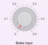
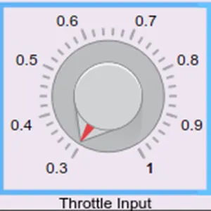
The model workflow process is same as the process of BAJA ATV model - mapped lookup table with Dashboard but the Throttle and Brake inputs are controlled by the user with the knob followed by the vehicle speed is given as feedback to the CVT Ratio lookup table.
Results:
ENGINE SPEED PLOT,
CVT SPEED PLOT,
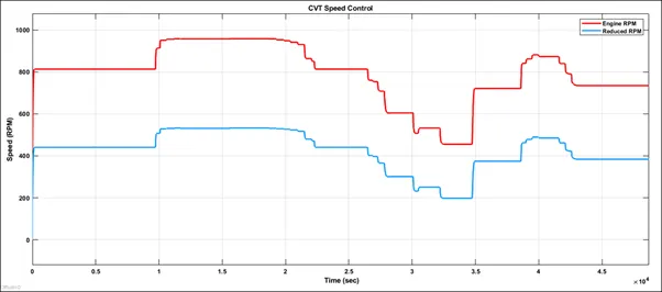
From the above graph we can understand that the throttle is applied (step up) and then kept constant then braking is applied (step down) then brake released so that the engine speedis increased with increase in throttle input.
INPUT vs VEHICLE SPEED,
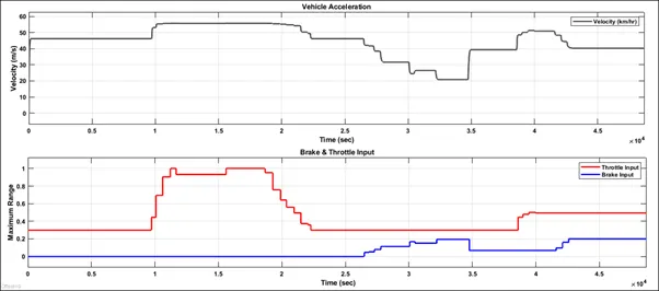
From the plot we can infer that when throttle is applied the vehicle speed increases and when brake is applied vehicle speed decreases simultaneously.
SIMULINK MODEL:
https://www.mathworks.com/matlabcentral/fileexchange/70576-baja-all-terrain-vehicle-atv-model