Project

AIM

To prepare a technical report explaining the model properties of an all-terrain vehicle by carrying out a system level simulation under different conditions.

OBJECTIVES

• Simulate the BAJA ATV model and understand the effect of Throttling input, Brake input and CVT ratio on the velocity of vehicle and position of vehicle body and CVT primary and secondary shaft speeds.
• Simulate the BAJA ATV model in real case scenarios by using Look up tables to determine the CVT ratio and understand the changes in vehicle velocity and CVT primary and secondary shaft speeds.

BAJA ATV MODEL

BAJA ATV simscape model with a Continuiosly Variable Transmission (CVT) is used as an all-terrain vehicle (ATV) in this simulation.All-terrain vehicle is also known as light utility vehicle. In India these types of vehicles are commonly used for agriculture purposes. In some countries it is used as a vehicle for racing.

Continious Variable Transmission (CVT)

The most important part of this transmission is pulley and belts. the power is transmitted from input shaft to output shaft with the help of these arranngement. The input Shaft is connected to the engine, so same power produced in the engine will be available in the input shaft. The belt is rotating in between the variators of the input shaft and the output shaft. The gap between the variators determines the diameter of the pulley. As the gap decreases, the effective diameter of pulley increases. This simple mechanism provides infinite gear ratio and speed will changes accordingly. This is the process behind Continious Variable Transmission.

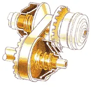
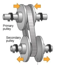
When the variator of the input shaft moves outwards and variator of output shaft moves inwards, then the radius of secondary pulley will be greater than that of primary pulley, which results in speed reduction.

If the variator of the input shaft moves inwards and variator of output shaft moves outwards then radius of primary pilley is greater than secondary pulley, which results in overdrive.

Simscape model for BAJA ATV (Open Loop System)

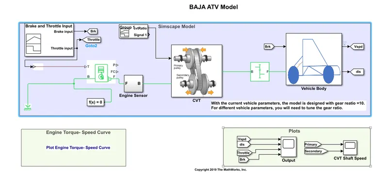
Model discription

a) Signal Builder: The brake and throttling input to the engine is provided with a signal builder and CVT ratio to the CVT is also made with signal builder.

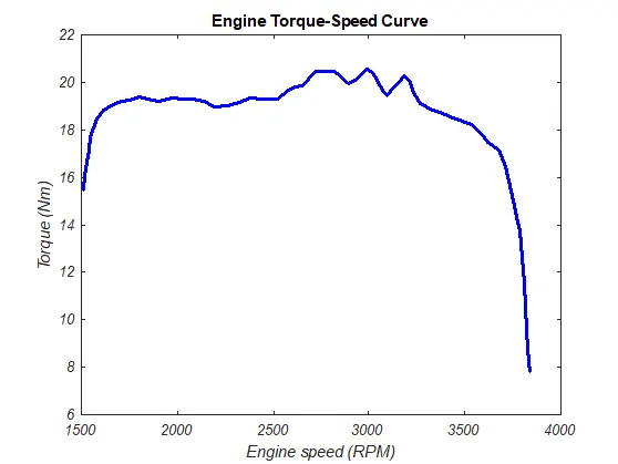
b) Generic Engine: It is used as an engine for BAJA ATV. It is basically represents a system level model of spark ignition and diesel engines suitable for all initial stages of modelling. We need to operate the engine at real case scenarios. The input data such as speed vector and Torque vector was taken by extracting the data from the Speed- Torque graph of a tipical BAJA engine. The Speed-Torque input to the engine is:

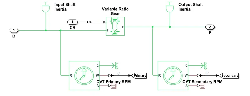
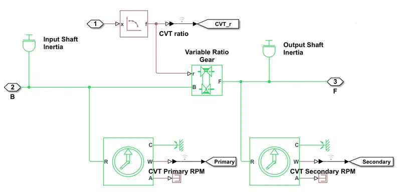
c) CVT Simscape Model: The CVT sub-system have an input shaft inertia and output shaft inertia which represents primary and secondary shaft pulley. To specify the gear ratio to CVT it has a variable gear ratio block. Two rotational sensors are provided to get the rpm of primary and secondary shaft. The subsystem model for the CVT is:

d) Vehicle Body: It represents a two axle vehicle body in longitudinal motion. The block accounts for body mass, aerodynamic drag, road incline and weight distribution between axle due to acceleration and road profile. The vehicle can have the same or different no of wheels on each axle. The default tyre values are used for this vehicle. A double shoe brake is provided for braking purpose. The input to the brake is given through the signal builder brake input. The subsystem for vehiclebody is:

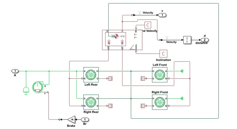
Simple Gear: A simple gear block is also connected between the Vehicle body and CVT inorder to specify the gear ratio to Vehicle. Here for the entire simulation the simple gear ratio was set to 10.

Case Study for BAJA ATV Model (Open Loop System)

a) Effect of Vehicle Mass on the Velocity of Vehicle

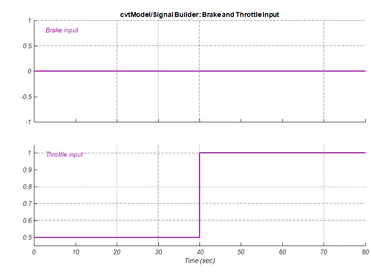
Here we are comparing vehicle with two different mass 100kg and 250kg. The Throttling input was initailly set to 0.5 for 40 sec then increases to full throttle =1 and Brake input was set to zero. The brake and throttling input to the system is:

The result obtained from the simulation is:

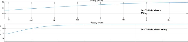
From the above graph it is clear that both the vehicle attaining maximum velocity of 59.5km/hr. But the vehicle with body mass 100kg attained maximum velocity with in 1.5 sec after increasing its throttling whereas the vehicle having bogy mass 250kg attained maximum velocity with in 3.5 sec after increasing the throttling. So vehicle with less mass attaining maximum velocity at faster rate than vehicle with high mass.

b) Effect of Throttling on the velocity of Vehicle and primary and secondary shaft speed

The throttling input to the system was intially set to 0.5 for first 40 sec then increases to full throttle =1 and brake input set to zero.

Result obtained for the velocity of the vehicle and primary and secondary shaft speeds are:

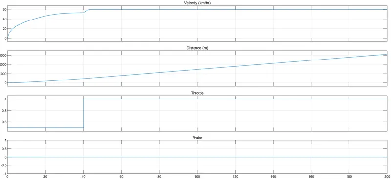
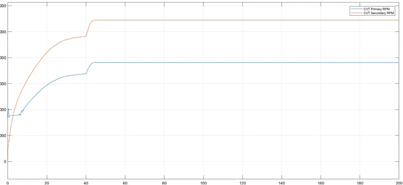
From the above fig it is cleared that, After 40 sec when the throttling input increases to full throttle = 1, The velocity of vehicle increase also increases and after certain time the vehicle is attaining its maximum velocity of approximately 59.5km/hr. Incase of primary and secondary Shaft speed also , As the throttling input increases both primary and secondary shaft rpm are increasing. The position of the vehicle is increasing linearly as the throttling increases. The brake input is zero in this case therefore no effect will be there.

c) Effect of CVT ratio in primary and secondary shaft speeds

The CVT ratio input to the CVT model provided with a signal builder. The input signal to the CVT is:

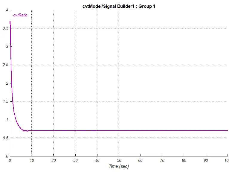
For 0 to 2.5 sec the CVT ratio is above 1 and after 2.5 sec CVT ratio is below 1 and it is maintaining an approximate constant value for the entire simulation.

The result obtained for the primary and secondary shaft speed is:

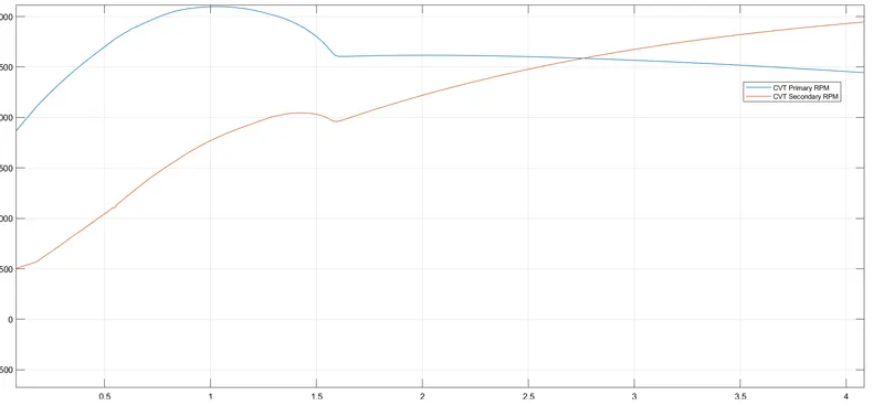
From the above graph it is cleared that, When the CVT ratio is more than 1 the RPM of primary is greater than secondary and when it is less than 1 the rpm of secondary is more than primary. So the primary shaft rpm and secondary shaft rpm is depands upon the change in the CVT ratio.If CVT ratio more than 1, speed of vehicle will decreases and if CVT ratio is less than 1, the speed of the vehicle increases.

d) Effect of Brake input on Velocity of vehicle

The brake input value was set to 0.25 and throttling input intially set to 0.5 for 40 sec then increses to full throttle=1, the results obtained for the primary and secondary shaft speed is :

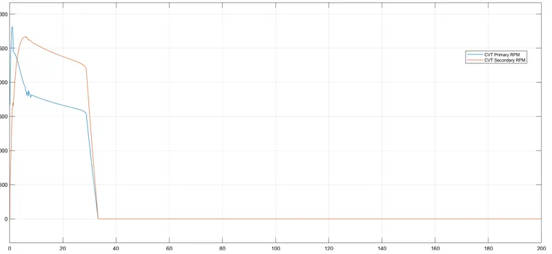
From the graph it found out that even though the throttling input increases to 1 after 40 sec, due to the braking input value of 0.25, the rpm of the primary and secondary shaft comes to zero. Therefore velocity of vehicle is zero in this case.

Case Study for BAJA ATV with Dashboard (Open loop system)

Inorder to operate the system in real manner, we are introducing a dashboard system where we can change the throttling input and brake input while the simulation is running.

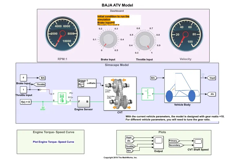
The results obtained from the simulations are:

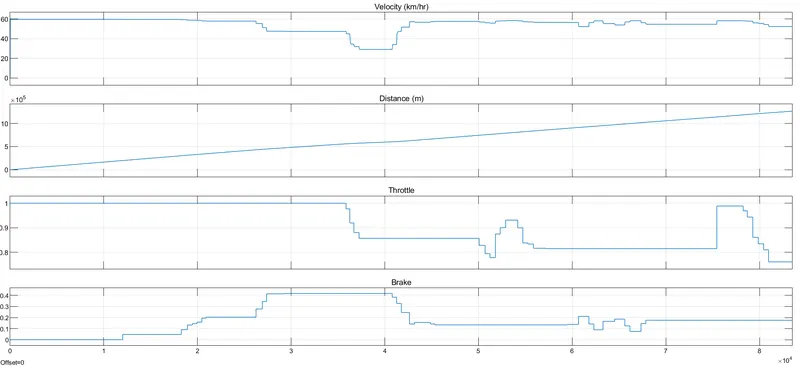
The simulation was done for a infinity sample time. From the above graph it is clear that, Initially the brake input is zero and throttling input is 1 i.e full throttle and maximum velocity of 59.5 km was attained by the vehicle. Once the braking is applied, gradually the velocity of the vehicle start to reduce and when the throttling was reduced we can see more reduction in the vehicle speed. At first the distance travelled by the vehicle is linear and increasing but as the throttling input and brake input changes, there is a variation from linearity which means more time require to reach the destination.

The result obtained for CVT primary and secondary shaft speed:

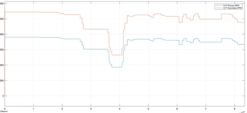
The primary CVT rpm and secondary CVT rpm were also changes as per the changes in the Throttling and Brake input.

So from the above system it is cleared that the Vehicle velocity depands upon Throttling input, Brake input, CVT ratio and the Vehicle mass etc. From the above we can understand that graph representing Velocity of the vehicle and the secondary CVT rpm shows nearly same because secondary shaft output is responsible for the movenment of the vehicle.

Case Study for BAJA ATV (Closed loop system)

In the open loop system we are giving some random values and checking the vehicle performance. Since it is not realistic because the CVT ratio depands upon vehicle velocity. So inorder to understand the BAJA ATV model in more realistic manner we are doing simulation with a closed loop system build with a Look up Table.

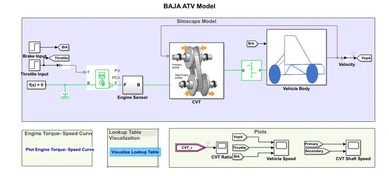
Key features of BAJA ATV Closed loop system are:

• The throttling input and Brake input are provided with two seperate step input. The throttling input was given with a step time of 40 sec and initial value was set to 0.3 and final value was set to 1. The brake input value was set to zero for the entire simulation.
• The CVT signal builder used in the open loop system was removed instead of that, a feedback was given to CVT block from the velocity of vehicle.
• Vehicle body remains same as that of open loop system.

A script was written to fetch the data of vehicle speed and CVT ratio from the open loop model and loaded to the look up table. The look up table visualization is:

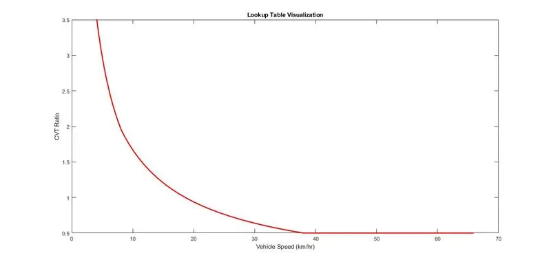
As we look into the CVT block, a Look up table is created in the subsystem of CVT block. So based on the data given to the Look up table.i.e velocity data, it will calculate the required amount of CVT ratio for the model. The subsytem for the CVT block with Look up table:

The simulation was run for a sample period of 0 to 200 sec. The throttling input was set to 0.3 intially and after 40 sec it will reaches its full throttle = 1, brake input det to zero.

The results obtained from the system for vehicle velocity is:

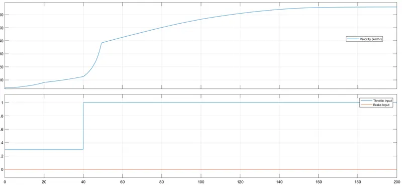
Here also we can see that, As the throttling increases the velocity of the system increases and after a certain period it reaches its maximun value = 65km/hr

The result of CVT ratio calculated from the model:

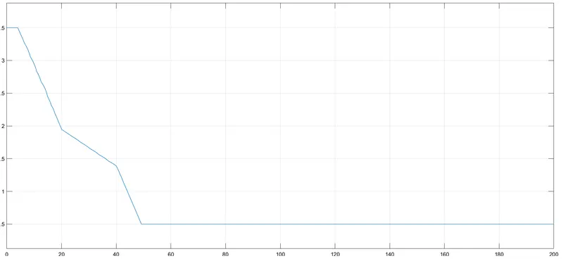
The above graph shows the CVT ratio calculated as per the data given into the Look up table. By comparing the graph of velocity and CVT ratio it found that for 0 to 40 sec the CVT ratio is above 1, therefore velocity of vehicle is less, after 40 sec the CVT ratio is less than 1 and velocity start increasing.

The result obtained for CVT primary and secondary shaft speed:

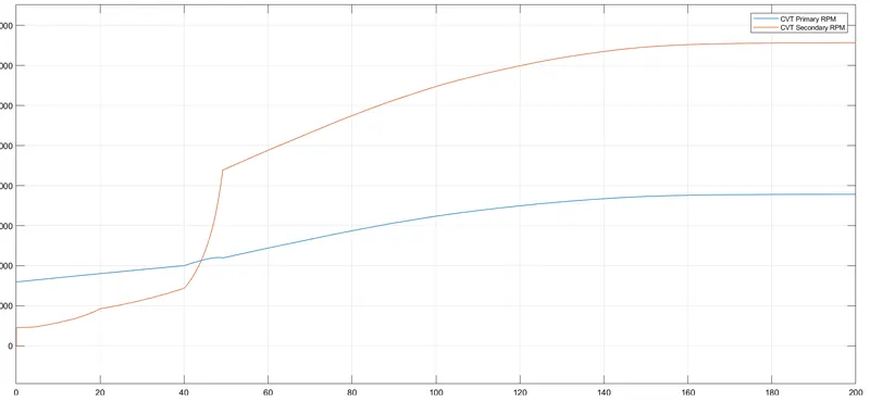
From the graph we can understand that, till 40 sec the rpm of secondary shaft is less than rpm of primary shaft due to higher CVT ratio. After 40 sec it is found that rpm of secondary increases and rpm of primary decreases due smaller CVT. One interesting thing is that graph of secondary rpm and graph of velocity of vehicle is same because rpm of secondary shaft is responsible movenment of vehicle. The engine rpm is getting as an input to the primary shaft, so the maximum primary rpm of 3840 is reached for the full throttle=1.

Case Study for BAJA ATV with Dashboard (Closed loop system)

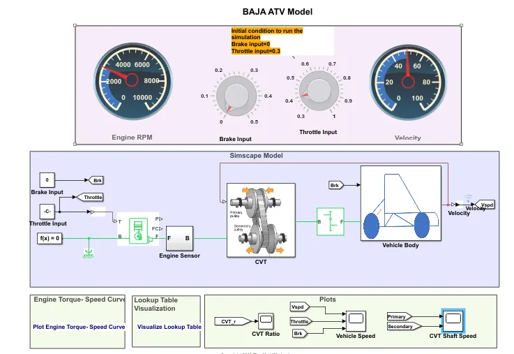
Here in this model with a dashboard, the simulation time was set to infinity, So user can change the value of throttling while the simulation is running. This model makes even more realistic as compared to above one. Here throttling input set to initail value of 0.3.

The result obtained from models are:

Vehicle velocity

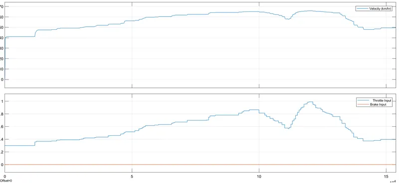
From graph we can see that initailly the throttling input to the system is around 0.3 and velocity of vehicle is around 40km/hr. As the throttling increases step by step, the velocity of vehicle also increased. Once the throttling reaches max value (i.e value=1) the velocity of vehiclealso reaches maximum value (i.e around 65km/hr).

CVT ratio calculated from the model

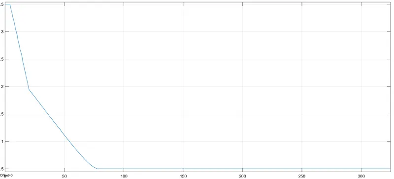
As we can see that CVT ratio is reaching its minimum value at a faster time( i.e within 80 sec) which means that Vehicle is attaining its maximum velocity with less amount of time.

The result obtained for CVT primary and secondary shaft speed

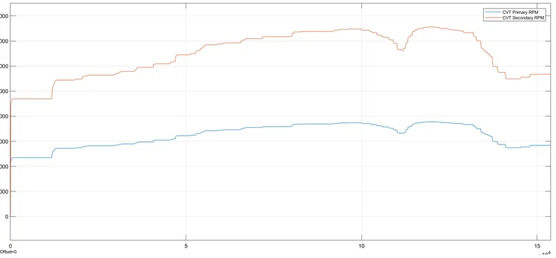
The graph indicate CVT primary rpm of input shaft and CVT secondary rpm of output shaft. The engine rpm is same as that of the CVT primary rpm. From the Torque -Speed graph, the maximum value of rpm input to the generic engine is around 3840 rpm. So CVT primary rpm attained a maximum rpm around 3840, when maximum throttle ia applied. Graph for CVT secondary rpm value is similar to Vehicle velocity because secondary rpm of output shaft is responsible for the vehicle to movenment.

FINAL RESULT

A system level simulation was carried out for an all terrain vehicle( BAJA ATV model). From the simulation results it is observed that the velocity of vehicle depands upon throttling input, brake input, CVT ratio, mass of the vehicle and CVT secondary rpm.

Simulation was carried out for BAJA ATV model made with look up table inorder to understand its realistic nature. CVT ratio was determined as per the feedback from the output velocity and graph was plotted.