Project

1. AIM: Modeling of a Contineously Variable Transmission (CVT) BAJA All-Terrain-Vehicle (ATV) and observe the vehicle speed with varitions in inputs like Throttle, Brake and vehicle body interface with axle system.
2. Intriduction:

The model is built by simulink basic blocks, Simscape blocks are Generic Engine to drive the vehicle, Variable Ratio Transmission to mimic the CVT, Simople Gear to covert the input speed to suitable output speed for vehicle and Vehicle body block and Tire(Magic Formula) bloks are used to build the vehicle. Also Dashboard blocks was used to monitor the basic parameters as shown in below figure.

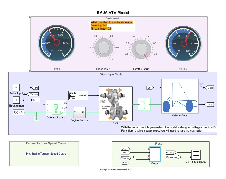
Generic Engine: it is a basically IC (Internal Combution) Engine. It produces the required torque coresponding to Throttle powerand which helps to drive the car.

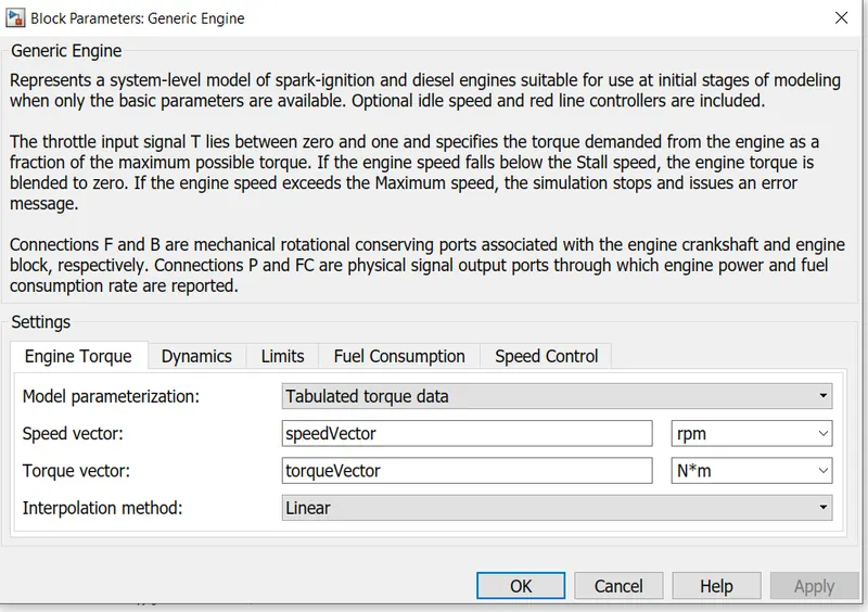
the input parameters for the Engine was choosen by Tabulated Torque data as shown in below figure.

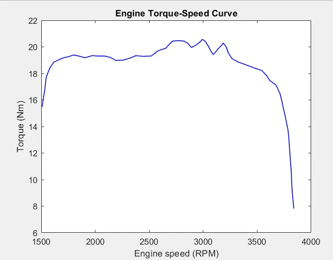
The Characteristics of speed, torque as below

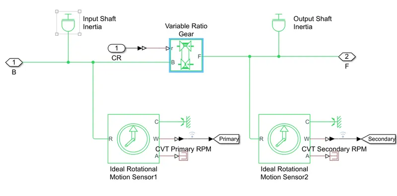
Output speed of Engine is measured by Ideal Rotational Motion Sensor and fed to the Dashboard of RPM1

CVT: is a type of automatic transmission that has an indefinite number of gear ratios. it changes the primary and secondary pully perimeter automaticall to change the gear ratio.

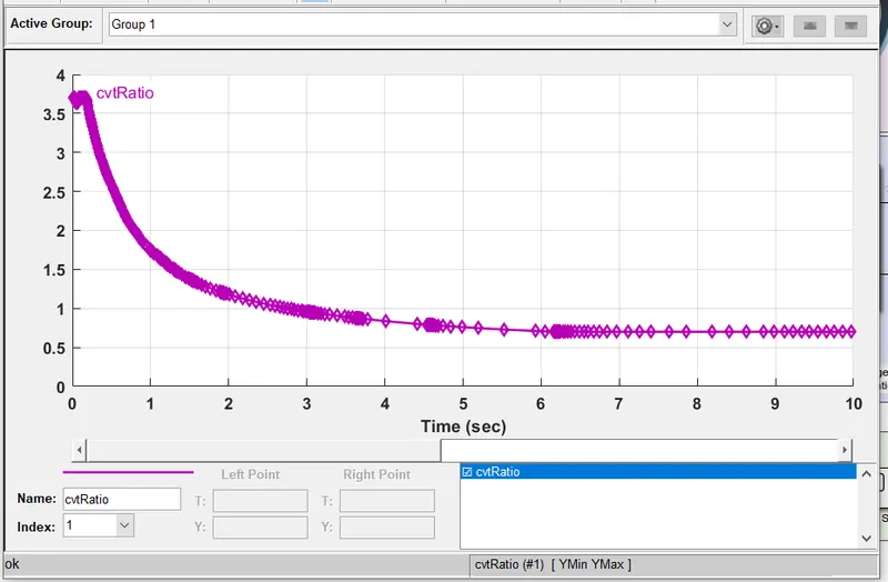
The engine output is fed to the Variable Transmission Ratio block and it its ratio is varied with help of CVT ratio data which is fed through Signal builder block, Primary and secondary rmp are measured by Ideal Rotational Motion Sensor and fed to scope for visualisation.

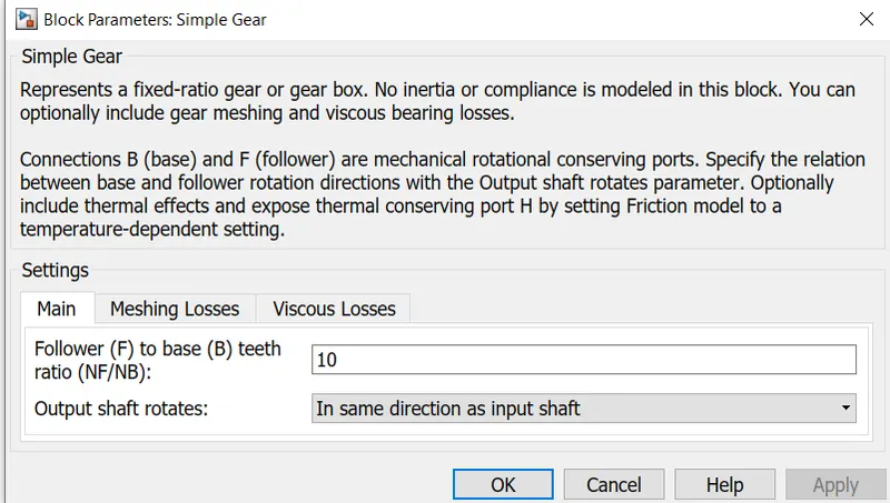
Simple Gear is used and its ratio is 10 to match the desired output parameters for vehicle body and tires, output shaft rotates in same direction as input shaft.

Vehicle Body and Tires: vehicle body and four(Two front and two rear) tires are properly connected to avoid errors during simulation as follows.

Wind, Beta effects are not condidered by giving zero input to them. Front tires are allowed to rotate freely and for rear tires shaft and brake powers are fed.

Double shoe Brake blockwas used to apply the brake mechanism as shown in figure.

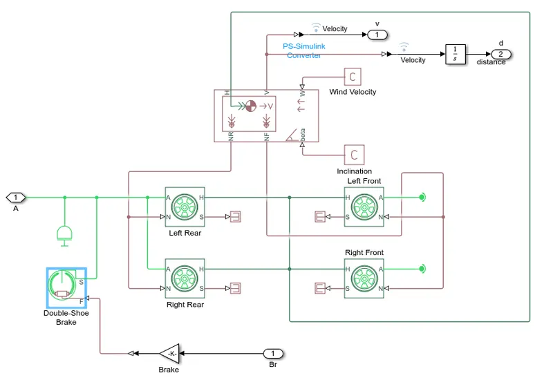
Slip of tires are termitad and vehicle velocity and distance traveled are monitored by scope.

Output Results and Observations:

Throttle=50% and Brake=0:

50% of throttle power is applied for engine without brake effect, the vehicle speed and distance travelled, CVT primary and secondary speed are as follows for run time of 70s.

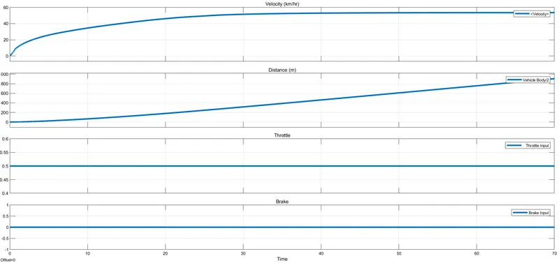
from graph-1 it is observed thet the vecle attains steady state speed of 50 kmph at 30sec and total distance travelled is around 900m.

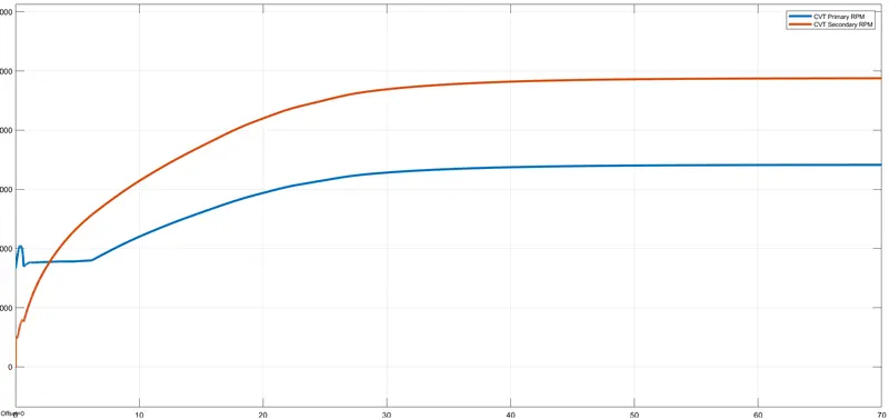
from graph-2 we can seethe CVT primary and secondary rpm, initially primary (blue colour) rpm is higher and after 4s secondary (Pink colour) rpm is high also we can see that at starting the rpm's are rapidly changed.

once vehicle reaches steady state there is no much change in CVT ratio and primary rpm is around 3400 rpm and secondary rpm is around 4900 rpm.

Throttle=50% and Brake=0.05:

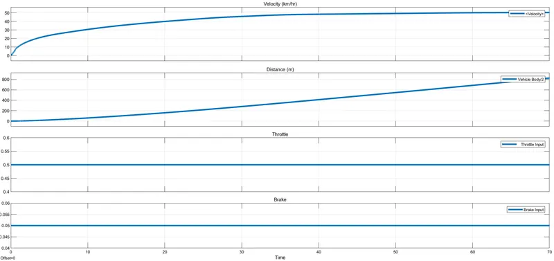
from graph-1 it is observed thet the vecle attains steady state speed of 50 kmph at 40sec (10s more compared to no brake),total distance travelled is around 800m (100m less compared to when No brake)

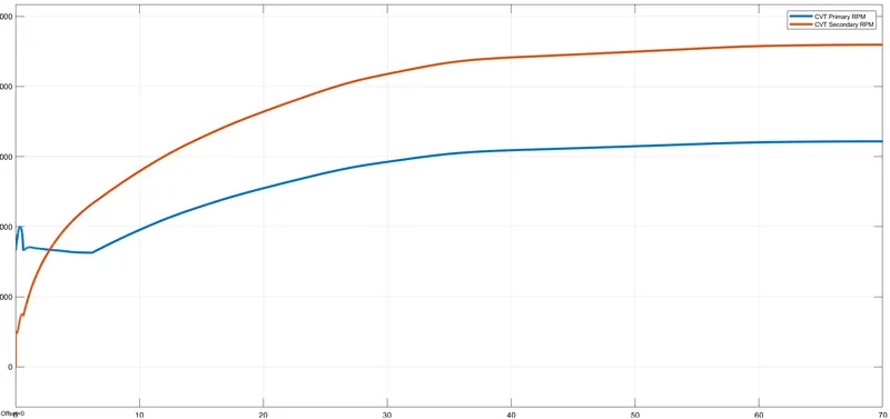
from graph-2 we can seethe CVT primary and secondary rpm, initially primary (blue colour) rpm is higher and after 4s secondary (Pink colour) rpm is high also we can see that at starting the rpm's are rapidly changed.

once vehicle reaches steady state there is no much change in CVT ratio and primary rpm is around 3100 rpm (3400rpm withput Brake) and secondary rpm is around 4500 rpm (4900rpm withput Brake).

Throttle=50% and Brake=0.1:

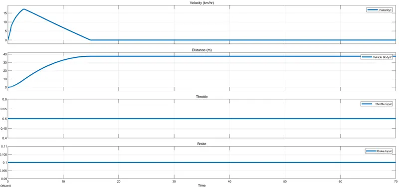
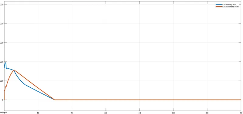
when 0.1 given to brake, the vehicle stopped acceleration after around 4s and deccelerated over 10s (from 5s to 15s) due to vehicle inertia and stopped after 15s. total distance travelled is 35m.

Throttle=75% and Brake=0.1:

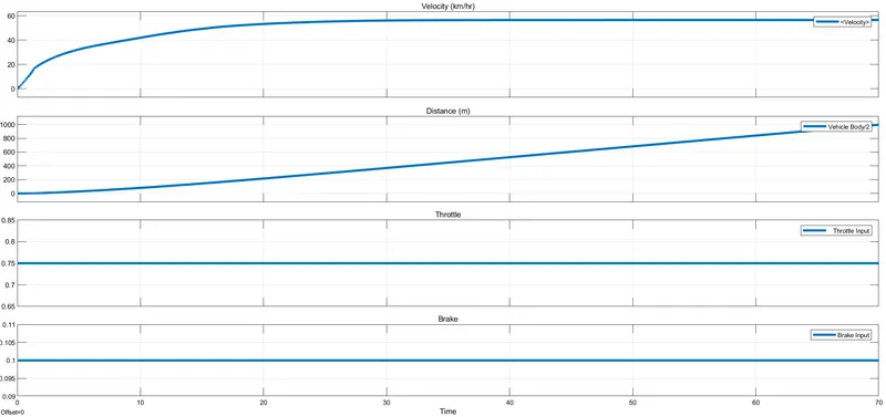
from graph-1 it is observed thet the vecle attains steady state speed of 59 kmph at 35sec (5s more compared to no brake and 50% throttle),total distance travelled is around 1100m (110m more compared to when No brake and 50% throttle)

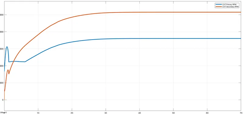
from graph-2 we can seethe CVT primary and secondary rpm, initially primary (blue colour) rpm is higher and after 4s secondary (Pink colour) rpm is high also we can see that at starting the rpm's are rapidly changed.

once vehicle reaches steady state there is no much change in CVT ratio and primary rpm is around 3650 rpm (3400rpm withput Brake) and secondary rpm is around 5100 rpm (4900rpm withput Brake).

Conclusion:

when vehicle is runnig with throttle and no brake, vehicle is moving smoothly and during stating thereis smaller peaks in CVT primary and secondary rpm values. when brake applied, it stoped the vehicle some time when break power is well enough, in other case it slowdowns the vehicle speed also reflects the more peaks in CVT primary and secondary rpm values. the effects can see in above MATLAB graphs.