Project 2_Rankine Cycle Simulator using MATLAB

About Rankine Cycle:

The rankine cycle is the ideal thermodynamic cycle which is the basic building block of the vapor power plants. It is widely used in the power plants. In the cycle, the heat is generated in the boiler by one of the fuel, converting the water into the steam. The steam then expands through a turbine to produde the work. The rankine cycle used in the power generation plants are, can be based on the renewable or nonrenewable based.

The following are the type of power plants used rankine cycle:

1: Coal-fueled

2: Nuclear-fueled

3: Oil-fueled

4. Biomass-fueled

5: Geothermal

6: Solar-concentrating

Following image describes the vapor power planrs operation based on fossile fuel.

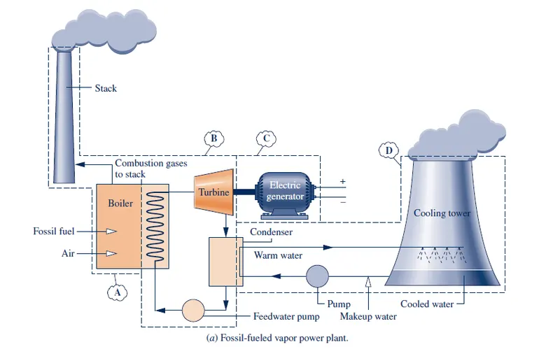
The section B in the above image is the example of the rankine cycle application in the industries. The subsystem displays in the B section is as follows:

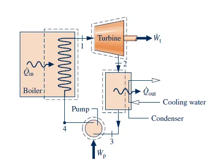
The same example has been used for develping rankine cycle simulator using MATLAB. The above cycle has 4 main components namely turbine, condenser, pump & boiler. The state points are mentioned in the image & energy transfers in the cycle are considered as positive in the direction of arrow.

Working of Rankine Cycle:

In the rankine cycle state point 1, the turbine expands the vapor received from the boiler at an elevated temperature & pressure has been used to produce work & discharged it to the condenser with low pressure at state point 2.

The heat has been transfered from the working fluid to the cooling water in the condenser which is flowing in the seperate stream. The temperature of the cooling water increases & the working fluid faces the phase change from the gaseous to liquid state and transfer the condensed fluid to the pump at state point 3.

The condensed liquid pumped into the high pressure boiler from the condenser. The boiler receives the fluid at state point 4 which completes the whole cycle. At state point 4, the fluid heated to the saturation point & evaporated in the boiler.

Main Code:

% Writing program to develop the simulator for the Rankine Cycle. 

% The Rankine cycle is an idealized thermodynamic cycle describing the
% process by which certain heat engines, such as steam turbines or
% reciprocating steam engines, allow mechanical work to be extracted from a
% fluid as it moves between a heat source and heat sink. (Source:
% Wikipedia)

% Inputs:
% Turbine Inlet temperature = 400° C
% Turbine Inlet Pressure = 30 bars
% Turbine Outlet Pressure = 0.05 bars = Condenser Inlet Pressure

% Objective:
% 1. Printing T-s & h-s diagram
% 2. Calculate net work output
% 3. Calculate Back work ratio

% Assumptions: Following assumptions are considered while developing the
% program
% 1. Each component at each state point is analyzed as a control volume at
% steady state.
% 2. All processes of the working fluid are internally reversible.
% 3. The turbine & pump operate adiabatically. 
% 4. Kinetic & potential energy  effects are negligible. 
% 5. Saturated vapor enters the turbine. Condensate exits the condenser as
% saturated liquid. 


close all; clear all; clc;

% Displaying Rankine Cycle Simulator title & processes
fprintf('%40snn','Rankine Cycle Simulator');
disp('1-2 is Isentropic Expansion in the Turbine')
disp('2-3 is Const Pressure Heat Rejection by the Condenser')
disp('3-4 is Isentropic Compression in the Pump')
disp('4-1 is Const Pressure Heat Addition by the Boiler')
disp(' ')
p_ini = input('Enter the Pressure at the Turbine Inlet, p1(in Bar): ');
t_ini = input('Enter the Temperature at the Turbine Inlet, t1(in Degree Celcius): ');
p_cond = input('Enter the Pressure at the Condenser, p2(in Bar): ');
disp(' ')
fprintf('%40s','Results');

% State variables at state point 1
p1 = 30; % Pressure (bar)
t1 = 400; % Temperature(degree C)
% Extracting variables from the Xsteam function file
% Enthalpy value for 30 bar pressure & 400 degree C temperature
h1 = XSteam('h_pT', p1,t1); % KJ/kg
% Entropy value for 30 bar pressure & enthalpy value at state point 1
s1 = XSteam('s_ph', p1, h1); % KJ/kg.K
% Printing State point & its variables
fprintf('nAt State Point 1:n')
fprintf(' P1 is : %f Barn', p1)
fprintf(' T1 is : %f Celciusn', t1)
fprintf(' H1 is : %f KJ/kg n', h1)
fprintf(' S1 is : %f KJ/kg.K n', s1)

% State variables at state point 2
p2 = 0.05; % Pressure (bar)
s2 = s1; % Constant entropy between process 1-2
% Extracting variables from the Xsteam function file
t2 = XSteam('T_ps', p2, s2); % Temperature(degree C)
sf2 = XSteam('sL_p', p2); % Entropy - Liquid state, value at p2
sg2 = XSteam('sV_p', p2); % Entropy - Vapor state, value at p2
hf2 = XSteam('hL_p', p2); % Enthalpy - Liquid state, value at p2
hg2 = XSteam('hV_p', p2); % Enthalpy - Vapor state, value at p2
% The quality at state point 2
x2 = ((s2 -sf2)/(sg2 - sf2));
% calculating enthalpy at state point 2
h2 = hf2 + x2*(hg2 - hf2);
% Printing State point & its variables
fprintf('nAt State Point 2:n')
fprintf(' P2 is : %f Barn', p2)
fprintf(' T2 is : %f Celciusn', t2)
fprintf(' H2 is : %f KJ/kg n', h2)
fprintf(' S2 is : %f KJ/kg.K n', s2)
fprintf(' X2 is : %f n', x2)

% State point 3
p3 = p2; % Constant pressure between process 2-3, heat rejection in condenser
t3 = t2; % Constant temperature between process 2-3
s3 = XSteam('sl_p', p3); % Entropy - Liquid state, value at p3
h3 = XSteam('hL_p', p3); % Enthalpy - Liquid state, value at p3
v3 = XSteam('v_ph', p3, h3); % Specific volume of liquid passing through the pump
% Printing State point & its variables
fprintf('nAt State Point 3:n')
fprintf(' P3 is : %f Barn', p3)
fprintf(' T3 is : %f Celciusn', t3)
fprintf(' H3 is : %f KJ/kg n', h3)
fprintf(' S3 is : %f KJ/kg.K n', s3)

% State point 4
s4 = s3; % Constant Entropy between process 3-4
p4 = p1; % working fluid flows constantly through boiler
% Calculating enthalpy 
h4 = h3 + v3*(p4 - p3);
t4 = XSteam('T_hs', h4, s4); % Temperature value from the XSteam using the enthalpy & entropy
% Printing State point & its variables
fprintf('nAt State Point 4:n')
fprintf(' P4 is : %f Barn', p4)
fprintf(' T4 is : %f Celciusn', t4)
fprintf(' H4 is : %f KJ/kg n', h4)
fprintf(' S4 is : %f KJ/kg.K n', s4)

% State point 5
p5 = p4; % Pressure
t5 = XSteam('Tsat_p', p5); % Temperature(degree C)
h5 = XSteam('hL_T', t5); % Enthalpy
s5 = XSteam('sL_p', p5); % Entropy

% State Point 6
t6 = t5; % Constant Temperature
p6 = XSteam('psat_T', t6); % Pressure
h6 = XSteam('hV_T', t6); % Enthalpy
s6 = XSteam('sV_T', t6); % Entropy

% Determining the process lines between state points
temp = linspace(1,t1,1000);

for i = 1:length(temp)
    s_l(i) = XSteam('sL_T', temp(i)); % Entropy (Liquid phase)
    s_v(i) = XSteam('sV_T', temp(i)); % Entropy (Vapor phase)
    h_l(i) = XSteam('hL_T', temp(i)); % Enthalpy (Liquid phase)
    h_v(i) = XSteam('hV_T', temp(i)); % Enthalpy (Vapor phase)
end

% Net heat into the system
Qin = h1 - h4;
% Net heat out of the system
Qout = h2 - h3;

% Turbine - Work done
Wt = h1 -h2;
% Printing Turbine work done value
fprintf('nWt is : %f KJ/kg', Wt)
% Pump - Work done
Wp = v3*(p4 - p3)*100; 
% Printing Pump work done value
fprintf('nWp is : %f KJ/kg', Wp)

% Net work output
Wn = Wt - Wp;
% Printing Net Work done value
fprintf('nWn is : %f KJ/kg', Wn)

% Back Work Ratio
bwr = Wp/Wt;

% Efficiency
eff = Wn/Qin; 
% Printing efficiency value
fprintf('nNtherm is : %f Percent', eff)

% Calculating Specific Steam Consumption (SSC)
ssc = 3600/Wt;
% Printing SSC value
fprintf('nS.S.C. is: %f kg/KWhn', ssc)

% Plotting
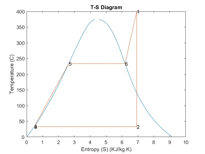
% T-s Diagram
figure(1)
% Plotting entropy for liquid & vapor phase
plot([s_l, s_v], [temp temp])
hold on
% Plotting lines between state points
plot([s1 s2 s3 s4 s5 s6 s1], [t1 t2 t3 t4 t5 t6 t1])
% Indicating state points on graph
text(s1, t1, '1') % State point 1
text(s2, t2, '2') % State point 2
text(s3, t3, '3') % State point 3
text(s4, t4, '4') % State point 4
text(s5, t5, '5') % State point 5
text(s6, t6, '6') % State point 6
hold off

title('T-S Diagram')
xlabel('Entropy (S) (KJ/kg.K)')
ylabel('Temperature (C)')

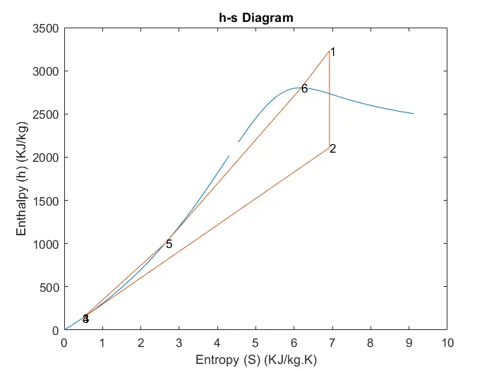
% Plotting h - s diagram
figure(2)
% Plotting entropy & enthalpy for liquid & vapor phase
plot([s_l, s_v], [h_l, h_v])
hold on
% Plotting lines between state points
plot([s1 s2 s3 s4 s5 s6 s1], [h1 h2 h3 h4 h5 h6 h1])
% Indicating state points on graph
text(s1, h1, '1') % State point 1
text(s2, h2, '2') % State point 2
text(s3, h3, '3') % State point 3
text(s4, h4, '4') % State point 4
text(s5, h5, '5') % State point 5
text(s6, h6, '6') % State point 6
hold off

title('h-s Diagram')
xlabel('Entropy (S) (KJ/kg.K)')
ylabel('Enthalpy (h) (KJ/kg)')

Graphs:

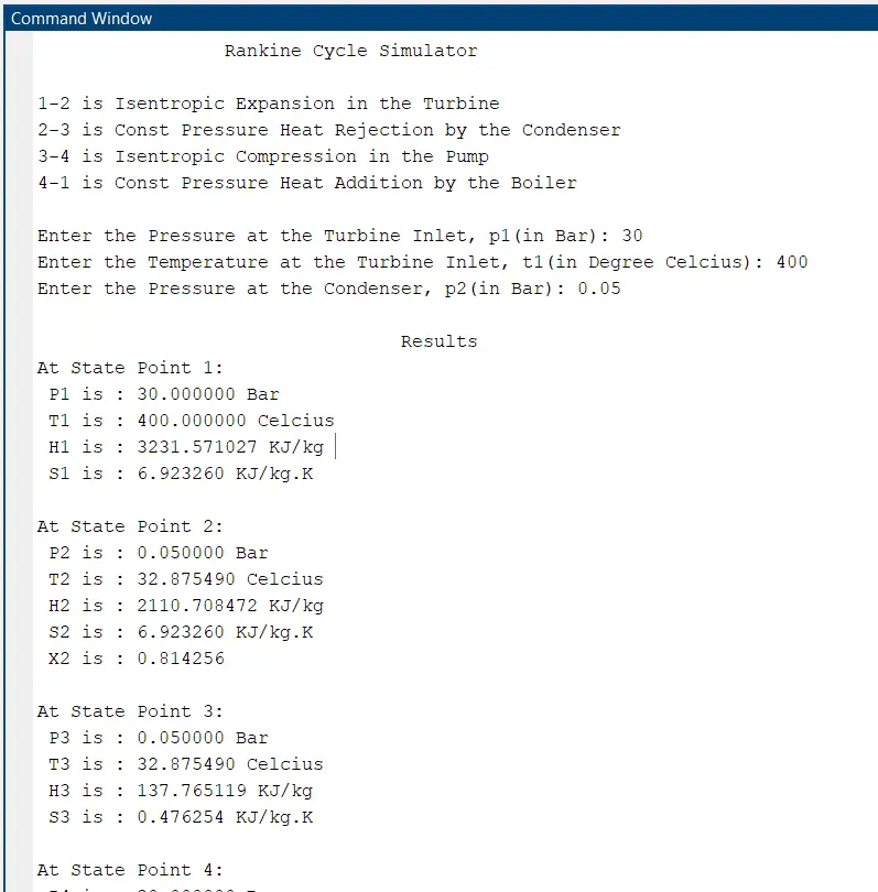
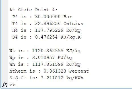
Results (Command Window Screenshots):

References:

Fundamentals of Engineering Thermodynamics book by Michael Moran